**Physically Based Rendering in Filament**

# About
This document is part of the [Filament project](https://github.com/google/filament). To report errors in this document please use the [project's issue tracker](https://github.com/google/filament/issues).
## Authors
- [Romain Guy](https://github.com/romainguy), [@romainguy](https://twitter.com/romainguy)
- [Mathias Agopian](https://github.com/pixelflinger), [@darthmoosious](https://twitter.com/darthmoosious)
# Overview
Filament is a physically based rendering (PBR) engine for Android. The goal of Filament is to offer a set of tools and APIs for Android developers that will enable them to create high quality 2D and 3D rendering with ease.
The goal of this document is to explain the equations and theory behind the material and lighting models used in Filament. This document is intended as a reference for contributors to Filament or developers interested in the inner workings of the engine. We will provide code snippets as needed to make the relationship between theory and practice as clear as possible.
This document is not intended as a design document. It focuses solely on algorithms and its content could be used to implement PBR in any engine. However, this document explains why we chose specific algorithms/models over others.
Unless noted otherwise, all the 3D renderings present in this document have been generated in-engine (prototype or production). Many of these 3D renderings were captured during the early stages of development of Filament and do not reflect the final quality.
## Principles
Real-time rendering is an active area of research and there is a large number of equations, algorithms and implementation to choose from for every single feature that needs to be implemented (the book *Rendering real-time shadows*, for instance, is a 400 pages summary of dozens of shadows rendering techniques). As such, we must first define our goals (or principles, to follow Brent Burley's seminal paper Physically-based shading at Disney [#Burley12]) before we can make informed decisions.
Real-time mobile performance
: Our primary goal is to design and implement a rendering system able to perform efficiently on mobile platforms. The primary target will be OpenGL ES 3.x class GPUs.
Quality
: Our rendering system will emphasize overall picture quality. We will however accept quality compromises to support low and medium performance GPUs.
Ease of use
: Artists need to be able to iterate often and quickly on their assets and our rendering system must allow them to do so intuitively. We must therefore provide parameters that are easy to understand (for instance, no specular power).
We also understand that not all developers have the luxury to work with artists. The physically based approach of our system will allow developers to craft visually plausible materials without the need to understand the theory behind our implementation.
For both artists and developers, our system will rely on as few parameters as possible to reduce trial and error and allow users to quickly master the material model.
In addition, any combination of parameter values should lead to physically plausible results. Physically implausible materials must be hard to create.
Familiarity
: Our system should use physical units everywhere possible: distances in meters or centimeters, color temperatures in Kelvin, light units in lumens or candelas, etc.
Flexibility
: A physically based approach must not preclude non-realistic rendering. User interfaces for instance will need unlit materials.
Deployment size
: While not directly related to the content of this document, it bears emphasizing our desire to keep the rendering library as small as possible so any application can bundle it without increasing the binary to undesirable sizes.
## Physically based rendering
We chose to adopt PBR for its benefits from an artistic and production efficient standpoints, and because it is compatible with our goals.
Physically based rendering is a rendering method that provides a more accurate representation of materials and how they interact with light when compared to traditional real-time models. The separation of materials and lighting at the core of the PBR method makes it easier to create realistic assets that look accurate in all lighting conditions.
# Notation
$$
\newcommand{NoL}{n \cdot l}
\newcommand{NoV}{n \cdot v}
\newcommand{NoH}{n \cdot h}
\newcommand{VoH}{v \cdot h}
\newcommand{LoH}{l \cdot h}
\newcommand{fNormal}{f_{0}}
\newcommand{fDiffuse}{f_d}
\newcommand{fSpecular}{f_r}
\newcommand{fX}{f_x}
\newcommand{aa}{\alpha^2}
\newcommand{fGrazing}{f_{90}}
\newcommand{schlick}{F_{Schlick}}
\newcommand{nior}{n_{ior}}
\newcommand{Ed}{E_d}
\newcommand{Lt}{L_{\bot}}
\newcommand{Lout}{L_{out}}
\newcommand{cosTheta}{\left< \cos \theta \right> }
$$
The equations found throughout this document use the symbols described in table [symbols].
Symbol | Definition
:---------------------------:|:---------------------------|
$v$ | View unit vector
$l$ | Incident light unit vector
$n$ | Surface normal unit vector
$h$ | Half unit vector between $l$ and $v$
$f$ | BRDF
$\fDiffuse$ | Diffuse component of a BRDF
$\fSpecular$ | Specular component of a BRDF
$\alpha$ | Roughness, remapped from using input `perceptualRoughness`
$\sigma$ | Diffuse reflectance
$\Omega$ | Spherical domain
$\fNormal$ | Reflectance at normal incidence
$\fGrazing$ | Reflectance at grazing angle
$\chi^+(a)$ | Heaviside function (1 if $a > 0$ and 0 otherwise)
$n_{ior}$ | Index of refraction (IOR) of an interface
$\left< \NoL \right>$ | Dot product clamped to [0..1]
$\left< a \right>$ | Saturated value (clamped to [0..1])
[Table [symbols]: Symbols definitions]
# Material system
The sections below describe multiple material models to simplify the description of various surface features such as anisotropy or the clear coat layer. In practice however some of these models are condensed into a single one. For instance, the standard model, the clear coat model and the anisotropic model can be combined to form a single, more flexible and powerful model. Please refer to the [Materials documentation](./Materials.md.html) to get a description of the material models as implemented in Filament.
## Standard model
The goal of our model is to represent standard material appearances. A material model is described mathematically by a BSDF (Bidirectional Scattering Distribution Function), which is itself composed of two other functions: the BRDF (Bidirectional Reflectance Distribution Function) and the BTDF (Bidirectional Transmittance Function).
Since we aim to model commonly encountered surfaces, our standard material model will focus on the BRDF and ignore the BTDF, or approximate it greatly. Our standard model will therefore only be able to correctly mimic reflective, isotropic, dielectric or conductive surfaces with short mean free paths.
The BRDF describes the surface response of a standard material as a function made of two terms:
- A diffuse component, or $f_d$
- A specular component, or $f_r$
The relationship between a surface, the surface normal, incident light and these terms is shown in figure [frFd] (we ignore subsurface scattering for now):
![Figure [frFd]: Interaction of the light with a surface using BRDF model with a diffuse term $ f_d $ and a specular term $ f_r $](images/diagram_fr_fd.png)
The complete surface response can be expressed as such:
$$\begin{equation}\label{brdf}
f(v,l)=f_d(v,l)+f_r(v,l)
\end{equation}$$
This equation characterizes the surface response for incident light from a single direction. The full rendering equation would require to integrate $l$ over the entire hemisphere.
Commonly encountered surfaces are usually not made of a flat interface so we need a model that can characterize the interaction of light with an irregular interface.
A microfacet BRDF is a good physically plausible BRDF for that purpose. Such BRDF states that surfaces are not smooth at a micro level, but made of a large number of randomly aligned planar surface fragments, called microfacets. Figure [microfacetVsFlat] shows the difference between a flat interface and an irregular interface at a micro level:
![Figure [microfacetVsFlat]: Irregular interface as modeled by a microfacet model (left) and flat interface (right)](images/diagram_microfacet.png)
Only the microfacets whose normal is oriented halfway between the light direction and the view direction will reflect visible light, as shown in figure [microfacets].
![Figure [microfacets]: Microfacets](images/diagram_macrosurface.png)
However, not all microfacets with a properly oriented normal will contribute reflected light as the BRDF takes into account masking and shadowing. This is illustrated in figure [microfacetShadowing].
![Figure [microfacetShadowing]: Masking and shadowing of microfacets](images/diagram_shadowing_masking.png)
A microfacet BRDF is heavily influenced by a _roughness_ parameter which describes how smooth (low roughness) or how rough (high roughness) a surface is at a micro level. The smoother the surface, the more facets are aligned and the more pronounced the reflected light is. The rougher the surface, the fewer facets are oriented towards the camera and incoming light is scattered away from the camera after reflection, giving a blurry aspect to the specular highlights.
Figure [roughness] shows surfaces of different roughness and how light interacts with them.
![Figure [roughness]: Varying roughness (from left to right, rough to smooth) and the resulting BRDF specular component lobe](images/diagram_roughness.png)
!!! Note: About roughness
The roughness parameter as set by the user is called `perceptualRoughness` in the shader snippets throughout this document. The variable called `roughness` is the `perceptualRoughness` with a remapping explained in section [Parameterization].
A microfacet model is described by the following equation (where x stands for the specular or diffuse component):
$$\begin{equation}
\fX(v,l) = \frac{1}{| \NoV | | \NoL |}
\int_\Omega D(m,\alpha) G(v,l,m) f_m(v,l,m) (v \cdot m) (l \cdot m) dm
\end{equation}$$
The term $D$ models the distribution of the microfacets (this term is also referred to as the NDF or Normal Distribution Function). This term plays a primordial role in the appearance of surfaces as shown in figure [roughness].
The term $G$ models the visibility (or occlusion or shadow-masking) of the microfacets.
Since this equation is valid for both the specular and diffuse components, the difference lies in the microfacet BRDF $f_m$.
It is important to note that this equation is used to integrate over the hemisphere at a _micro level_:
![Figure [microLevel]: Modeling the surface response at a single point requires an integration at the micro level](images/diagram_micro_vs_macro.png)
The diagram above shows that at a macro level, the surfaces is considered flat. This helps simplify our equations by assuming that a shaded fragment lit from a single direction corresponds to a single point at the surface.
At a micro level however, the surface is not flat and we cannot assume a single ray of light anymore (we can however assume that the incident rays are parallel). Since the micro facets will scatter the light in different directions given a bundle of parallel incident rays, we must integrate the surface response over a hemisphere, noted m in the above diagram.
It is obviously not practical to compute the full integration over the microfacets hemisphere for each shaded fragment. We will therefore rely on approximations of the integration for both the specular and diffuse components.
## Dielectrics and conductors
To better understand some of the equations and behaviors shown below, we must first clearly understand the difference between metallic (conductor) and non-metallic (dielectric) surfaces.
We saw earlier that when incident light hits a surface governed by a BRDF, the light is reflected as two separate components: the diffuse reflectance and the specular reflectance. The modelization of this behavior is straightforward as shown in figure [bsdfBrdf].
![Figure [bsdfBrdf]: Modelization of the BRDF part of a BSDF](images/diagram_fr_fd.png)
This modelization is a simplification of how the light actually interacts with the surface. In reality, part of the incident light will penetrate the surface, scatter inside, and exit the surface again as diffuse reflectance. This phenomenon is illustrated in figure [diffuseScattering].
![Figure [diffuseScattering]: Scattering of diffuse light](images/diagram_scattering.png)
Here lies the difference between conductors and dielectrics. There is no subsurface scattering occurring with purely metallic materials, which means there is no diffuse component (and we will see later that this has an influence on the perceived color of the specular component). Scattering happens in dielectrics, which means they have both specular and diffuse components.
To properly modelize the BRDF we must therefore distinguish between dielectrics and conductors (scattering not shown for clarity), as shown in figure [dielectricConductor].
![Figure [dielectricConductor]: BRDF modelization for dielectric and conductor surfaces](images/diagram_brdf_dielectric_conductor.png)
## Energy conservation
Energy conservation is one of the key components of a good BRDF for physically based rendering. An energy conservative BRDF states that the total amount of specular and diffuse reflectance energy is less than the total amount of incident energy. Without an energy conservative BRDF, artists must manually ensure that the light reflected off a surface is never more intense than the incident light.
## Specular BRDF
For the specular term, $f_r$ is a mirror BRDF that can be modeled with the Fresnel law, noted $F$ in the Cook-Torrance approximation of the microfacet model integration:
$$\begin{equation}
f_r(v,l) = \frac{D(h, \alpha) G(v, l, \alpha) F(v, h, f0)}{4(\NoV)(\NoL)}
\end{equation}$$
Given our real-time constraints, we must use an approximation for the three terms $D$, $G$ and $F$. [#Karis13a] has compiled a great list of formulations for these three terms that can be used with the Cook-Torrance specular BRDF. The sections that follow describe the equations we picked for these terms.
### Normal distribution function (specular D)
[#Burley12] observed that long-tailed normal distribution functions (NDF) are a good fit for real-world surfaces. The GGX distribution described in [#Walter07] is a distribution with long-tailed falloff and short peak in the highlights, with a simple formulation suitable for real-time implementations. It is also a popular model, equivalent to the Trowbridge-Reitz distribution, in modern physically based renderers.
$$\begin{equation}
D_{GGX}(h,\alpha) = \frac{\aa}{\pi ( (\NoH)^2 (\aa - 1) + 1)^2}
\end{equation}$$
The GLSL implementation of the NDF, shown in listing [specularD], is simple and efficient.
~~~~~~~~~~~~~~~~~~~~~~~~~~~~~~~~~~~~~~
float D_GGX(float NoH, float roughness) {
float a = NoH * roughness;
float k = roughness / (1.0 - NoH * NoH + a * a);
return k * k * (1.0 / PI);
}
~~~~~~~~~~~~~~~~~~~~~~~~~~~~~~~~~~~~~~
[Listing [specularD]: Implementation of the specular D term in GLSL]
We can improve this implementation by using half precision floats. This optimization requires changes to the original equation as there are two problems when computing $1 - (\NoH)^2$ in half-floats. First, this computation suffers from floating point cancellation when $(\NoH)^2$ is close to 1 (highlights). Secondly $\NoH$ does not have enough precision around 1.
The solution involves Lagrange's identity:
$$\begin{equation}
| a \times b |^2 = |a|^2 |b|^2 - (a \cdot b)^2
\end{equation}$$
Since both $n$ and $h$ are unit vectors, $|n \times h|^2 = 1 - (\NoH)^2$. This allows us to compute $1 - (\NoH)^2$ directly with half precision floats by using a simple cross product. Listing [specularDfp16] shows the final optimized implementation.
~~~~~~~~~~~~~~~~~~~~~~~~~~~~~~~~~~~~~~
#define MEDIUMP_FLT_MAX 65504.0
#define saturateMediump(x) min(x, MEDIUMP_FLT_MAX)
float D_GGX(float roughness, float NoH, const vec3 n, const vec3 h) {
vec3 NxH = cross(n, h);
float a = NoH * roughness;
float k = roughness / (dot(NxH, NxH) + a * a);
float d = k * k * (1.0 / PI);
return saturateMediump(d);
}
~~~~~~~~~~~~~~~~~~~~~~~~~~~~~~~~~~~~~~
[Listing [specularDfp16]: Implementation of the specular D term in GLSL optimized for fp16]
### Geometric shadowing (specular G)
Eric Heitz showed in [#Heitz14] that the Smith geometric shadowing function is the correct and exact $G$ term to use. The Smith formulation is the following:
$$\begin{equation}
G(v,l,\alpha) = G_1(l,\alpha) G_1(v,\alpha)
\end{equation}$$
$G_1$ can in turn follow several models, and is commonly set to the GGX formulation:
$$\begin{equation}
G_1(v,\alpha) = G_{GGX}(v,\alpha) = \frac{2 (\NoV)}{\NoV + \sqrt{\aa + (1 - \aa) (\NoV)^2}}
\end{equation}$$
The full Smith-GGX formulation thus becomes:
$$\begin{equation}
G(v,l,\alpha) = \frac{2 (\NoL)}{\NoL + \sqrt{\aa + (1 - \aa) (\NoL)^2}} \frac{2 (\NoV)}{\NoV + \sqrt{\aa + (1 - \aa) (\NoV)^2}}
\end{equation}$$
We can observe that the dividends $2 (\NoL)$ and $2 (n \cdot v)$ allow us to simplify the original function $f_r$ by introducing a visibility function $V$:
$$\begin{equation}
f_r(v,l) = D(h, \alpha) V(v, l, \alpha) F(v, h, f_0)
\end{equation}$$
Where:
$$\begin{equation}
V(v,l,\alpha) = \frac{G(v, l, \alpha)}{4 (\NoV) (\NoL)} = V_1(l,\alpha) V_1(v,\alpha)
\end{equation}$$
And:
$$\begin{equation}
V_1(v,\alpha) = \frac{1}{\NoV + \sqrt{\aa + (1 - \aa) (\NoV)^2}}
\end{equation}$$
Heitz notes however that taking the height of the microfacets into account to correlate masking and shadowing leads to more accurate results. He defines the height-correlated Smith function thusly:
$$\begin{equation}
G(v,l,h,\alpha) = \frac{\chi^+(\VoH) \chi^+(\LoH)}{1 + \Lambda(v) + \Lambda(l)}
\end{equation}$$
$$\begin{equation}
\Lambda(m) = \frac{-1 + \sqrt{1 + \aa tan^2(\theta_m)}}{2} = \frac{-1 + \sqrt{1 + \aa \frac{(1 - cos^2(\theta_m))}{cos^2(\theta_m)}}}{2}
\end{equation}$$
Replacing $cos(\theta_m)$ by $\NoV$, we obtain:
$$\begin{equation}
\Lambda(v) = \frac{1}{2} \left( \frac{\sqrt{\aa + (1 - \aa)(\NoV)^2}}{\NoV} - 1 \right)
\end{equation}$$
From which we can derive the visibility function:
$$\begin{equation}
V(v,l,\alpha) = \frac{0.5}{\NoL \sqrt{(\NoV)^2 (1 - \aa) + \aa} + \NoV \sqrt{(\NoL)^2 (1 - \aa) + \aa}}
\end{equation}$$
The GLSL implementation of the visibility term, shown in listing [specularV], is a bit more expensive than we would like since it requires two `sqrt` operations.
~~~~~~~~~~~~~~~~~~~~~~~~~~~~~~~~~~~~~~
float V_SmithGGXCorrelated(float NoV, float NoL, float roughness) {
float a2 = roughness * roughness;
float GGXV = NoL * sqrt(NoV * NoV * (1.0 - a2) + a2);
float GGXL = NoV * sqrt(NoL * NoL * (1.0 - a2) + a2);
return 0.5 / (GGXV + GGXL);
}
~~~~~~~~~~~~~~~~~~~~~~~~~~~~~~~~~~~~~~
[Listing [specularV]: Implementation of the specular V term in GLSL]
We can optimize this visibility function by using an approximation after noticing that all the terms under the square roots are squares and that all the terms are in the $[0..1]$ range:
$$\begin{equation}
V(v,l,\alpha) = \frac{0.5}{\NoL (\NoV (1 - \alpha) + \alpha) + \NoV (\NoL (1 - \alpha) + \alpha)}
\end{equation}$$
This approximation is mathematically wrong but saves two square root operations and is good enough for real-time mobile applications, as shown in listing [approximatedSpecularV].
~~~~~~~~~~~~~~~~~~~~~~~~~~~~~~~~~~~~~~
float V_SmithGGXCorrelatedFast(float NoV, float NoL, float roughness) {
float a = roughness;
float GGXV = NoL * (NoV * (1.0 - a) + a);
float GGXL = NoV * (NoL * (1.0 - a) + a);
return 0.5 / (GGXV + GGXL);
}
~~~~~~~~~~~~~~~~~~~~~~~~~~~~~~~~~~~~~~
[Listing [approximatedSpecularV]: Implementation of the approximated specular V term in GLSL]
[#Hammon17] proposes the same approximation based on the same observation that the square root can be removed. It does so by rewriting the expressions as _lerps_:
$$\begin{equation}
V(v,l,\alpha) = \frac{0.5}{lerp(2 (\NoL) (\NoV), \NoL + \NoV, \alpha)}
\end{equation}$$
### Fresnel (specular F)
The Fresnel effect plays an important role in the appearance of physically based materials. This effect models the fact that the amount of light the viewer sees reflected from a surface depends on the viewing angle. Large bodies of water are a perfect way to experience this phenomenon, as shown in figure [fresnelLake]. When looking at the water straight down (at normal incidence) you can see through the water. However, when looking further out in the distance (at grazing angle, where perceived light rays are getting parallel to the surface), you will see the specular reflections on the water become more intense.
The amount of light reflected depends not only on the viewing angle, but also on the index of refraction (IOR) of the material. At normal incidence (perpendicular to the surface, or 0 degree angle), the amount of light reflected back is noted $\fNormal$ and can be derived from the IOR as we will see in section [Reflectance remapping]. The amount of light reflected back at grazing angle is noted $\fGrazing$ and approaches 100% for smooth materials.
![Figure [fresnelLake]: The Fresnel effect is particularly evident on large bodies of water](images/photo_fresnel_lake.jpg)
More formally, the Fresnel term defines how light reflects and refracts at the interface between two different media, or the ratio of reflected and transmitted energy. [#Schlick94] describes an inexpensive approximation of the Fresnel term for the Cook-Torrance specular BRDF:
$$\begin{equation}
F_{Schlick}(v,h,\fNormal,\fGrazing) = \fNormal + (\fGrazing - \fNormal)(1 - \VoH)^5
\end{equation}$$
The constant $\fNormal$ represents the specular reflectance at normal incidence and is achromatic for dielectrics, and chromatic for metals. The actual value depends on the index of refraction of the interface. The GLSL implementation of this term requires the use of a `pow`, as shown in listing [specularF], which can be replaced by a few multiplications.
~~~~~~~~~~~~~~~~~~~~~~~~~~~~~~~~~~~~~~
vec3 F_Schlick(float u, vec3 f0, float f90) {
return f0 + (vec3(f90) - f0) * pow(1.0 - u, 5.0);
}
~~~~~~~~~~~~~~~~~~~~~~~~~~~~~~~~~~~~~~
[Listing [specularF]: Implementation of the specular F term in GLSL]
This Fresnel function can be seen as interpolating between the incident specular reflectance and the reflectance at grazing angles, represented here by $\fGrazing$. Observation of real world materials show that both dielectrics and conductors exhibit achromatic specular reflectance at grazing angles and that the Fresnel reflectance is 1.0 at 90 degrees. A more correct $\fGrazing$ is discussed in section [Specular occlusion].
Using $\fGrazing$ set to 1, the Schlick approximation for the Fresnel term can be optimized for scalar operations by refactoring the code slightly. The result is shown in listing [scalarSpecularF].
~~~~~~~~~~~~~~~~~~~~~~~~~~~~~~~~~~~~~~
vec3 F_Schlick(float u, vec3 f0) {
float f = pow(1.0 - u, 5.0);
return f + f0 * (1.0 - f);
}
~~~~~~~~~~~~~~~~~~~~~~~~~~~~~~~~~~~~~~
[Listing [scalarSpecularF]: Scalar optimization of the specular F term in GLSL]
## Diffuse BRDF
In the diffuse term, $f_m$ is a Lambertian function and the diffuse term of the BRDF becomes:
$$\begin{equation}
\fDiffuse(v,l) = \frac{\sigma}{\pi} \frac{1}{| \NoV | | \NoL |}
\int_\Omega D(m,\alpha) G(v,l,m) (v \cdot m) (l \cdot m) dm
\end{equation}$$
Our implementation will instead use a simple Lambertian BRDF that assumes a uniform diffuse response over the microfacets hemisphere:
$$\begin{equation}
\fDiffuse(v,l) = \frac{\sigma}{\pi}
\end{equation}$$
In practice, the diffuse reflectance $\sigma$ is multiplied later, as shown in listing [diffuseBRDF].
~~~~~~~~~~~~~~~~~~~~~~~~~~~~~~~~~~~~~~
float Fd_Lambert() {
return 1.0 / PI;
}
vec3 Fd = diffuseColor * Fd_Lambert();
~~~~~~~~~~~~~~~~~~~~~~~~~~~~~~~~~~~~~~
[Listing [diffuseBRDF]: Implementation of the diffuse Lambertian BRDF in GLSL]
The Lambertian BRDF is obviously extremely efficient and delivers results close enough to more complex models.
However, the diffuse part would ideally be coherent with the specular term and take into account the surface roughness. Both the Disney diffuse BRDF [#Burley12] and Oren-Nayar model [#Oren94] take the roughness into account and create some retro-reflection at grazing angles. Given our constraints we decided that the extra runtime cost does not justify the slight increase in quality. This sophisticated diffuse model also renders image-based and spherical harmonics more difficult to express and implement.
For completeness, the Disney diffuse BRDF expressed in [#Burley12] is the following:
$$\begin{equation}
\fDiffuse(v,l) = \frac{\sigma}{\pi} \schlick(n,l,1,\fGrazing) \schlick(n,v,1,\fGrazing)
\end{equation}$$
Where:
$$\begin{equation}
\fGrazing=0.5 + 2 \cdot \alpha cos^2(\theta_d)
\end{equation}$$
~~~~~~~~~~~~~~~~~~~~~~~~~~~~~~~~~~~~~~
float F_Schlick(float u, float f0, float f90) {
return f0 + (f90 - f0) * pow(1.0 - u, 5.0);
}
float Fd_Burley(float NoV, float NoL, float LoH, float roughness) {
float f90 = 0.5 + 2.0 * roughness * LoH * LoH;
float lightScatter = F_Schlick(NoL, 1.0, f90);
float viewScatter = F_Schlick(NoV, 1.0, f90);
return lightScatter * viewScatter * (1.0 / PI);
}
~~~~~~~~~~~~~~~~~~~~~~~~~~~~~~~~~~~~~~
[Listing [diffuseBRDF]: Implementation of the diffuse Disney BRDF in GLSL]
Figure [lambert_vs_disney] shows a comparison between a simple Lambertian diffuse BRDF and the higher quality Disney diffuse BRDF, using a fully rough dielectric material. For comparison purposes, the right sphere was mirrored. The surface response is very similar with both BRDFs but the Disney one exhibits some nice retro-reflections at grazing angles (look closely at the left edge of the spheres).
![Figure [lambert_vs_disney]: Comparison between the Lambertian diffuse BRDF (left) and the Disney diffuse BRDF (right)](images/diagram_lambert_vs_disney.png)
We could allow artists/developers to choose the Disney diffuse BRDF depending on the quality they desire and the performance of the target device. It is important to note however that the Disney diffuse BRDF is not energy conserving as expressed here.
## Standard model summary
**Specular term**: a Cook-Torrance specular microfacet model, with a GGX normal distribution function, a Smith-GGX height-correlated visibility function, and a Schlick Fresnel function.
**Diffuse term**: a Lambertian diffuse model.
The full GLSL implementation of the standard model is shown in listing [glslBRDF].
~~~~~~~~~~~~~~~~~~~~~~~~~~~~~~~~~~~~~~
float D_GGX(float NoH, float a) {
float a2 = a * a;
float f = (NoH * a2 - NoH) * NoH + 1.0;
return a2 / (PI * f * f);
}
vec3 F_Schlick(float u, vec3 f0) {
return f0 + (vec3(1.0) - f0) * pow(1.0 - u, 5.0);
}
float V_SmithGGXCorrelated(float NoV, float NoL, float a) {
float a2 = a * a;
float GGXL = NoV * sqrt((-NoL * a2 + NoL) * NoL + a2);
float GGXV = NoL * sqrt((-NoV * a2 + NoV) * NoV + a2);
return 0.5 / (GGXV + GGXL);
}
float Fd_Lambert() {
return 1.0 / PI;
}
void BRDF(...) {
vec3 h = normalize(v + l);
float NoV = abs(dot(n, v)) + 1e-5;
float NoL = clamp(dot(n, l), 0.0, 1.0);
float NoH = clamp(dot(n, h), 0.0, 1.0);
float LoH = clamp(dot(l, h), 0.0, 1.0);
// perceptually linear roughness to roughness (see parameterization)
float roughness = perceptualRoughness * perceptualRoughness;
float D = D_GGX(NoH, roughness);
vec3 F = F_Schlick(LoH, f0);
float V = V_SmithGGXCorrelated(NoV, NoL, roughness);
// specular BRDF
vec3 Fr = (D * V) * F;
// diffuse BRDF
vec3 Fd = diffuseColor * Fd_Lambert();
// apply lighting...
}
~~~~~~~~~~~~~~~~~~~~~~~~~~~~~~~~~~~~~~
[Listing [glslBRDF]: Evaluation of the BRDF in GLSL]
## Improving the BRDFs
We mentioned in section [Energy conservation] that energy conservation is one of the key components of a good BRDF. Unfortunately the BRDFs explored previously suffer from two problems that we will examine below.
### Energy gain in diffuse reflectance
The Lambert diffuse BRDF does not account for the light that reflects at the surface and that is therefore not able to participate in the diffuse scattering event.
[TODO: talk about the issue with fr+fd]
### Energy loss in specular reflectance
The Cook-Torrance BRDF we presented earlier attempts to model several events at the microfacet level but does so by accounting for a single bounce of light. This approximation can cause a loss of energy at high roughness, the surface is not energy preserving. Figure [singleVsMultiBounce] shows why this loss of energy occurs. In the single bounce (or single scattering) model, a ray of light hitting the surface can be reflected back onto another microfacet and thus be discarded because of the masking and shadowing term. If we however account for multiple bounces (multiscattering), the same ray of light might escape the microfacet field and be reflected back towards the viewer.
![Figure [singleVsMultiBounce]: Single scattering (left) vs multiscattering](images/diagram_single_vs_multi_scatter.png)
Based on this simple explanation, we can intuitively deduce that the rougher a surface is, the higher the chances are that energy gets lost because of the failure to account for multiple scattering events. This loss of energy appears to darken rough materials. Metallic surfaces are particularly affected because all of their reflectance is specular. This darkening effect is illustrated in figure [metallicRoughEnergyLoss]. With multiscattering, energy preservation can be achieved, as shown in figure [metallicRoughEnergyPreservation].
![Figure [metallicRoughEnergyLoss]: Darkening increases with roughness due to single scattering](images/material_metallic_energy_loss.png)
![Figure [metallicRoughEnergyPreservation]: Energy preservation with multiscattering](images/material_metallic_energy_preservation.png)
We can use a white furnace, a uniform lighting environment set to pure white, to validate the energy preservation property of a BRDF. When energy preservation is achieved, a purely reflective metallic surface ($\fNormal = 1$) should be indistinguishable from the background, no matter the roughness of said surface. Figure [whiteFurnaceLoss] shows what such a surface looks like with the specular BRDF presented in the previous sections. The loss of energy as the roughness increases is obvious. In contrast, figure [whiteFurnacePreservation] shows that accounting for multiscattering events addresses the energy loss.
![Figure [whiteFurnaceLoss]: Darkening increases with roughness due to single scattering](images/material_furnace_energy_loss.png)
![Figure [whiteFurnacePreservation]: Energy preservation with multiscattering](images/material_furnace_energy_preservation.png)
Multiple-scattering microfacet BRDFs are discussed in depth in [#Heitz16]. Unfortunately this paper only presents a stochastic evaluation of the multiscattering BRDF. This solution is therefore not suitable for real-time rendering. Kulla and Conty present a different approach in [#Kulla17]. Their idea is to add an energy compensation term as an additional BRDF lobe shown in equation $\ref{energyCompensationLobe}$:
$$\begin{equation}\label{energyCompensationLobe}
f_{ms}(l,v) = \frac{(1 - E(l)) (1 - E(v)) F_{avg}^2 E_{avg}}{\pi (1 - E_{avg}) (1 - F_{avg}(1 - E_{avg}))}
\end{equation}$$
Where $E$ is the directional albedo of the specular BRDF $f_r$, with $\fNormal$ set to 1:
$$\begin{equation}
E(l) = \int_{\Omega} f(l,v) (\NoV) dv
\end{equation}$$
The term $E_{avg}$ is the cosine-weighted average of $E$:
$$\begin{equation}
E_{avg} = 2 \int_0^1 E(\mu) \mu d\mu
\end{equation}$$
Similarly, $F_{avg}$ is the cosine-weighted average of the Fresnel term:
$$\begin{equation}
F_{avg} = 2 \int_0^1 F(\mu) \mu d\mu
\end{equation}$$
Both terms $E$ and $E_{avg}$ can be precomputed and stored in lookup tables. while $F_{avg}$ can be greatly simplified when the Schlick approximation is used:
$$\begin{equation}\label{averageFresnel}
F_{avg} = \frac{1 + 20 \fNormal}{21}
\end{equation}$$
This new lobe is combined with the original single scattering lobe, previously noted $f_r$:
$$\begin{equation}
f_{r}(l,v) = f_{ss}(l,v) + f_{ms}(l,v)
\end{equation}$$
In [#Lagarde18], with credit to Emmanuel Turquin, Lagarde and Golubev make the observation that equation $\ref{averageFresnel}$ can be simplified to $\fNormal$. They also propose to apply energy compensation by adding a scaled GGX specular lobe:
$$\begin{equation}\label{energyCompensation}
f_{ms}(l,v) = \fNormal \frac{1 - E(l)}{E(l)} f_{ss}(l,v)
\end{equation}$$
The key insight is that $E(l)$ can not only be precomputed but also shared with image-based lighting pre-integration. The multiscattering energy compensation formula thus becomes:
$$\begin{equation}\label{scaledEnergyCompensationLobe}
f_r(l,v) = f_{ss}(l,v) + \fNormal \left( \frac{1}{r} - 1 \right) f_{ss}(l,v)
\end{equation}$$
Where $r$ is defined as:
$$\begin{equation}
r = \int_{\Omega} D(l,v) V(l,v) \left< \NoL \right> dl
\end{equation}$$
We can implement specular energy compensation at a negligible cost if we store $r$ in the DFG lookup table presented in section [Image based lights]. Listing [energyCompensationImpl] shows that the implementation is a direct conversion of equation $\ref{scaledEnergyCompensationLobe}$.
~~~~~~~~~~~~~~~~~~~~~~~~~~~~~~~~~~~~~~
vec3 energyCompensation = 1.0 + f0 * (1.0 / dfg.y - 1.0);
// Scale the specular lobe to account for multiscattering
Fr *= pixel.energyCompensation;
~~~~~~~~~~~~~~~~~~~~~~~~~~~~~~~~~~~~~~
[Listing [energyCompensationImpl]: Implementation of the energy compensation specular lobe]
Please refer to section [Image based lights] and section [Pre-integration for multiscattering] to learn how the DFG lookup table is derived and computed.
## Parameterization
Disney's material model described in [#Burley12] is a good starting point but its numerous parameters makes it impractical for real-time implementations. In addition, we would like our standard material model to be easy to understand and easy to use for both artists and developers.
### Standard parameters
Table [standardParameters] describes the list of parameters that satisfy our constraints.
Parameter | Definition
---------------------:|:---------------------
**BaseColor** | Diffuse albedo for non-metallic surfaces, and specular color for metallic surfaces
**Metallic** | Whether a surface appears to be dielectric (0.0) or conductor (1.0). Often used as a binary value (0 or 1)
**Roughness** | Perceived smoothness (0.0) or roughness (1.0) of a surface. Smooth surfaces exhibit sharp reflections
**Reflectance** | Fresnel reflectance at normal incidence for dielectric surfaces. This replaces an explicit index of refraction
**Emissive** | Additional diffuse albedo to simulate emissive surfaces (such as neons, etc.) This parameter is mostly useful in an HDR pipeline with a bloom pass
**Ambient occlusion** | Defines how much of the ambient light is accessible to a surface point. It is a per-pixel shadowing factor between 0.0 and 1.0. This parameter will be discussed in more details in the lighting section
[Table [standardParameters]: Parameters of the standard model]
Figure [material_parameters] shows how the metallic, roughness and reflectance parameters affect the appearance of a surface.
![Figure [material_parameters]: From top to bottom: varying metallic, varying dielectric roughness, varying metallic roughness, varying reflectance](images/material_parameters.png)
### Types and ranges
It is important to understand the type and range of the different parameters of our material model, described in table [standardParametersTypes].
Parameter | Type and range
---------------------:|:---------------------
**BaseColor** | Linear RGB [0..1]
**Metallic** | Scalar [0..1]
**Roughness** | Scalar [0..1]
**Reflectance** | Scalar [0..1]
**Emissive** | Linear RGB [0..1] + exposure compensation
**Ambient occlusion** | Scalar [0..1]
[Table [standardParametersTypes]: Range and type of the standard model's parameters]
Note that the types and ranges described here are what the shader will expect. The API and/or tools UI could and should allow to specify the parameters using other types and ranges when they are more intuitive for artists.
For instance, the base color could be expressed in sRGB space and converted to linear space before being sent off to the shader. It can also be useful for artists to express the metallic, roughness and reflectance parameters as gray values between 0 and 255 (black to white).
Another example: the emissive parameter could be expressed as a color temperature and an intensity, to simulate the light emitted by a black body.
### Remapping
To make the standard material model easier and more intuitive to use for artists, we must remap the parameters _baseColor_, _roughness_ and _reflectance_.
#### Base color remapping
The base color of a material is affected by the "metallicness" of said material. Dielectrics have achromatic specular reflectance but retain their base color as the diffuse color. Conductors on the other hand use their base color as the specular color and do not have a diffuse component.
The lighting equations must therefore use the diffuse color and $\fNormal$ instead of the base color. The diffuse color can easily be computed from the base color, as show in listing [baseColorToDiffuse].
~~~~~~~~~~~~~~~~~~~~~~~~~~~~~~~~~~~~~~
vec3 diffuseColor = (1.0 - metallic) * baseColor.rgb;
~~~~~~~~~~~~~~~~~~~~~~~~~~~~~~~~~~~~~~
[Listing [baseColorToDiffuse]: Conversion of base color to diffuse in GLSL]
#### Reflectance remapping
**Dielectrics**
The Fresnel term relies on $\fNormal$, the specular reflectance at normal incidence angle, and is achromatic for dielectrics. We will use the remapping for dielectric surfaces described in [#Lagarde14] :
$$\begin{equation}
\fNormal = 0.16 \cdot reflectance^2
\end{equation}$$
The goal is to map $\fNormal$ onto a range that can represent the Fresnel values of both common dielectric surfaces (4% reflectance) and gemstones (8% to 16%). The mapping function is chosen to yield a 4% Fresnel reflectance value for an input reflectance of 0.5 (or 128 on a linear RGB gray scale). Figure [reflectance] show those common values and how they relate to the mapping function.
![Figure [reflectance]: Common reflectance values](images/diagram_reflectance.png)
If the index of refraction is known (for instance, an air-water interface has an IOR of 1.33), the Fresnel reflectance can be calculated as follows:
$$\begin{equation}\label{fresnelEquation}
\fNormal(n_{ior}) = \frac{(\nior - 1)^2}{(\nior + 1)^2}
\end{equation}$$
And if the reflectance value is known, we can compute the corresponding IOR:
$$\begin{equation}
n_{ior} = \frac{2}{1 - \sqrt{\fNormal}} - 1
\end{equation}$$
Table [commonMatReflectance] describes acceptable Fresnel reflectance values for various types of materials (no real world material has a value under 2%).
Material | Reflectance | IOR | Linear value
--------------------------:|:-----------------|:-----------------|:----------------
Water | 2% | 1.33 | 0.35
Fabric | 4% to 5.6% | 1.5 to 1.62 | 0.5 to 0.59
Common liquids | 2% to 4% | 1.33 to 1.5 | 0.35 to 0.5
Common gemstones | 5% to 16% | 1.58 to 2.33 | 0.56 to 1.0
Plastics, glass | 4% to 5% | 1.5 to 1.58 | 0.5 to 0.56
Other dielectric materials | 2% to 5% | 1.33 to 1.58 | 0.35 to 0.56
Eyes | 2.5% | 1.38 | 0.39
Skin | 2.8% | 1.4 | 0.42
Hair | 4.6% | 1.55 | 0.54
Teeth | 5.8% | 1.63 | 0.6
Default value | 4% | 1.5 | 0.5
[Table [commonMatReflectance]: Reflectance of common materials (source: Real-Time Rendering 4th Edition)]
Table [fNormalMetals] lists the $\fNormal$ values for a few metals. The values are given in sRGB and must be used as the base color in our material model. Please refer to the annex, section [Specular color], for an explanation of how these sRGB colors are computed from measured data.
Metal | $\fNormal$ in sRGB | Hexadecimal | Color
----------:|:-------------------:|:------------:|-------------------------------------------------------
Silver | 0.97, 0.96, 0.91 | #f7f4e8 |
Aluminum | 0.91, 0.92, 0.92 | #e8eaea |
Titanium | 0.76, 0.73, 0.69 | #c1baaf |
Iron | 0.77, 0.78, 0.78 | #c4c6c6 |
Platinum | 0.83, 0.81, 0.78 | #d3cec6 |
Gold | 1.00, 0.85, 0.57 | #ffd891 |
Brass | 0.98, 0.90, 0.59 | #f9e596 |
Copper | 0.97, 0.74, 0.62 | #f7bc9e |
[Table [fNormalMetals]: $\fNormal$ for common metals]
All materials have a Fresnel reflectance of 100% at grazing angles so we will set $\fGrazing$ in the following way when evaluating the specular BRDF $\fSpecular$:
$$\begin{equation}
\fGrazing = 1.0
\end{equation}$$
Figure [grazing_reflectance] shows a red plastic ball. If you look closely at the edges of the sphere, you will be able to notice the achromatic specular reflectance at grazing angles.
![Figure [grazing_reflectance]: The specular reflectance becomes achromatic at grazing angles](images/material_grazing_reflectance.png)
**Conductors**
The specular reflectance of metallic surfaces is chromatic:
$$\begin{equation}
\fNormal = baseColor \cdot metallic
\end{equation}$$
Listing [fNormal] shows how $\fNormal$ is computed for both dielectric and metallic materials. It shows that the color of the specular reflectance is derived from the base color in the metallic case.
~~~~~~~~~~~~~~~~~~~~~~~~~~~~~~~~~~~~~~
vec3 f0 = 0.16 * reflectance * reflectance * (1.0 - metallic) + baseColor * metallic;
~~~~~~~~~~~~~~~~~~~~~~~~~~~~~~~~~~~~~~
[Listing [fNormal]: Computing $\fNormal$ for dielectric and metallic materials in GLSL]
#### Roughness remapping and clamping
The roughness set by the user, called `perceptualRoughness` here, is remapped to a perceptually linear range using the following formulation:
$$\begin{equation}
\alpha = perceptualRoughness^2
\end{equation}$$
Figure [roughness_remap] shows a silver metallic surface with increasing roughness (from 0.0 to 1.0), using the unmodified roughness value (bottom) and the remapped value (top).
![Figure [roughness_remap]: Roughness remapping comparison: perceptually linear roughness (top) and roughness (bottom)](images/material_roughness_remap.png)
Using this visual comparison, it is obvious that the remapped roughness is easier to understand by artists and developers. Without this remapping, shiny metallic surfaces would have to be confined to a very small range between 0.0 and 0.05.
Brent Burley made similar observations in his presentation [#Burley12]. After experimenting with other remappings (cubic and quadratic mappings for instance), we have reached the conclusion that this simple square remapping delivers visually pleasing and intuitive results while being cheap for real-time applications.
Last but not least, it is important to note that the roughness parameters is used in various computations at runtime where limited floating point precision can become an issue. For instance, _mediump_ precision floats are often implemented as half-floats (fp16) on mobile GPUs.
This cause problems when computing small values like $\frac{1}{perceptualRoughness^4}$ in our lighting equations (roughness squared in the GGX computation). The smallest value that can be represented as a half-float is $2^{-14}$ or $6.1 \times 10^{-5}$. To avoid divisions by 0 on devices that do not support denormals, the result of $\frac{1}{roughness^4}$ must therefore not be lower than $6.1 \times 10^{-5}$. To do so, we must clamp the roughness to 0.089, which gives us $6.274 \times 10^{-5}$.
Denormals should also be avoided to prevent performance drops. The roughness can also not be set to 0 to avoid obvious divisions by 0.
Since we also want specular highlights to have a minimum size (a roughness close to 0 creates almost invisible highlights), we should clamp the roughness to a safe range in the shader. This clamping has the added benefit of correcting specular aliasing[^frostbiteRoughnessClamp] that can appear for low roughness values.
[^frostbiteRoughnessClamp]: The Frostbite engine clamps the roughness of analytical lights to 0.045 to reduce specular aliasing. This is possible when using single precision floats (fp32).
### Blending and layering
As noted in [#Burley12] and [#Neubelt13], this model allows for robust blending between different materials by simply interpolating the different parameters. In particular, this allows to layer different materials using simple masks.
For instance, figure [materialBlending] shows how the studio Ready at Dawn used material blending and layering in _The Order: 1886_ to create complex appearances from a library of simple materials (gold, copper, wood, rust, etc.).
![Figure [materialBlending]: Material blending and layering. Source: Ready at Dawn Studios](images/material_blending.png)
The blending and layering of materials is effectively an interpolation of the various parameters of the material model. Figure [material_interpolation] show an interpolation between shiny metallic chrome and rough red plastic. While the intermediate blended materials make little physical sense, they look plausible.
![Figure [material_interpolation]: Interpolation from shiny chrome (left) to rough red plastic (right)](images/material_interpolation.png)
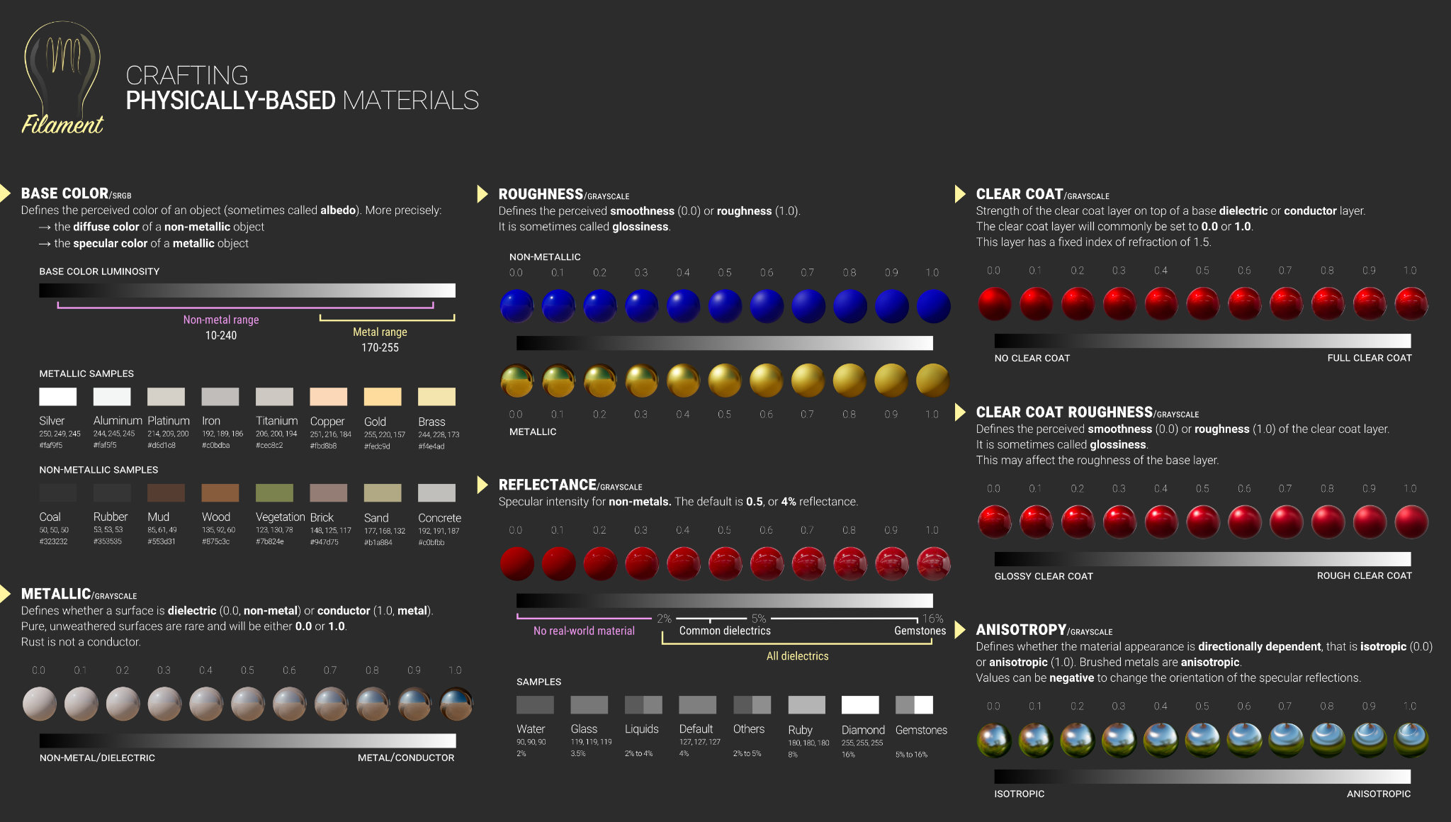
### Crafting physically based materials
Designing physically based materials is fairly easy once you understand the nature of the four main parameters: base color, metallic, roughness and reflectance.
We provide a [useful chart/reference guide](./Material%20Properties.pdf) to help artists and developers craft their own physically based materials.
In addition, here is a quick summary of how to use our material model:
All materials
: **Base color** should be devoid of lighting information, except for micro-occlusion.
**Metallic** is almost a binary value. Pure conductors have a metallic value of 1 and pure dielectrics have a metallic value of 0. You should try to use values close at or close to 0 and 1. Intermediate values are meant for transitions between surface types (metal to rust for instance).
Non-metallic materials
: **Base color** represents the reflected color and should be an sRGB value in the range 50-240 (strict range) or 30-240 (tolerant range).
**Metallic** should be 0 or close to 0.
**Reflectance** should be set to 127 sRGB (0.5 linear, 4% reflectance) if you cannot find a proper value. Do not use values under 90 sRGB (0.35 linear, 2% reflectance).
Metallic materials
: **Base color** represents both the specular color and reflectance. Use values with a luminosity of 67% to 100% (170-255 sRGB). Oxidized or dirty metals should use a lower luminosity than clean metals to take into account the non-metallic components.
**Metallic** should be 1 or close to 1.
**Reflectance** is ignored (calculated from the base color).
## Clear coat model
The standard material model described previously is a good fit for isotropic surfaces made of a single layer. Multi-layer materials are unfortunately fairly common, particularly materials with a thin translucent layer over a standard layer. Real world examples of such materials include car paints, soda cans, lacquered wood, acrylic, etc.
![Figure [materialClearCoat]: Comparison of a blue metallic surface under the standard material model (left) and the clear coat model (right)](images/material_clear_coat.png)
A clear coat layer can be simulated as an extension of the standard material model by adding a second specular lobe, which implies evaluating a second specular BRDF. To simplify the implementation and parameterization, the clear coat layer will always be isotropic and dielectric. The base layer can be anything allowed by the standard model (dielectric or conductor).
Since incoming light will traverse the clear coat layer, we must also take the loss of energy into account as shown in figure [clearCoatModel]. Our model will however not simulate inter reflection and refraction behaviors.
![Figure [clearCoatModel]: Clear coat surface model](images/diagram_clear_coat.png)
### Clear coat specular BRDF
The clear coat layer will be modeled using the same Cook-Torrance microfacet BRDF used in the standard model. Since the clear coat layer is always isotropic and dielectric, with low roughness values (see section [Clear coat parameterization]), we can choose cheaper DFG terms without notably sacrificing visual quality.
A survey of the terms listed in [#Karis13a] and [#Burley12] shows that the Fresnel and NDF terms we already use in the standard model are not computationally more expensive than other terms. [#Kelemen01] describes a much simpler term that can replace our Smith-GGX visibility term:
$$\begin{equation}
V(l,h) = \frac{1}{4(\LoH)^2}
\end{equation}$$
This masking-shadowing function is not physically based, as shown in [#Heitz14], but its simplicity makes it desirable for real-time rendering.
In summary, our clear coat BRDF is a Cook-Torrance specular microfacet model, with a GGX normal distribution function, a Kelemen visibility function, and a Schlick Fresnel function. Listing [kelemen] shows how trivial the GLSL implementation is.
~~~~~~~~~~~~~~~~~~~~~~~~~~~~~~~~~~~~~~
float V_Kelemen(float LoH) {
return 0.25 / (LoH * LoH);
}
~~~~~~~~~~~~~~~~~~~~~~~~~~~~~~~~~~~~~~
[Listing [kelemen]: Implementation of the Kelemen visibility term in GLSL]
**Note on the Fresnel term**
The Fresnel term of the specular BRDF requires $\fNormal$, the specular reflectance at normal incidence angle. This parameter can be computed from an index of refraction of an interface. We will assume that our clear coat layer is made of polyurethane, a common compound [used in coatings and varnishes](https://en.wikipedia.org/wiki/List_of_polyurethane_applications#Varnish), or similar. An air-polyurethane interface [has an IOR of 1.5](http://www.clearpur.com/transparent-polyurethanes/), from which we can deduce $\fNormal$:
$$\begin{equation}
\fNormal(1.5) = \frac{(1.5 - 1)^2}{(1.5 + 1)^2} = 0.04
\end{equation}$$
This corresponds to a Fresnel reflectance of 4% that we know is associated with common dielectric materials.
### Integration in the surface response
Because we must take into account the loss of energy caused by the addition of the clear coat layer, we can reformulate the BRDF from equation $\ref{brdf}$ thusly:
$$\begin{equation}
f(v,l)=\fDiffuse(v,l) (1 - F_c) + \fSpecular(v,l) (1 - F_c) + f_c(v,l)
\end{equation}$$
Where $F_c$ is the Fresnel term of the clear coat BRDF and $f_c$ the clear coat BRDF
### Clear coat parameterization
The clear coat material model encompasses all the parameters previously defined for the standard material mode, plus two parameters described in table [clearCoatParameters].
Parameter | Definition
----------------------:|:---------------------
**ClearCoat** | Strength of the clear coat layer. Scalar between 0 and 1
**ClearCoatRoughness** | Perceived smoothness or roughness of the clear coat layer. Scalar between 0 and 1
[Table [clearCoatParameters]: Clear coat model parameters]
The clear coat roughness parameter is remapped and clamped in a similar way to the roughness parameter of the standard material.
Figure [clearCoat] and figure [clearCoatRoughness] show how the clear coat parameters affect the appearance of a surface.
![Figure [clearCoat]: Clear coat varying from 0.0 (left) to 1.0 (right) with metallic set to 1.0 and roughness to 0.8](images/material_clear_coat1.png)
![Figure [clearCoatRoughness]: Clear coat roughness varying from 0.0 (left) to 1.0 (right) with metallic set to 1.0, roughness to 0.8 and clear coat to 1.0](images/material_clear_coat2.png)
Listing [clearCoatBRDF] shows the GLSL implementation of the clear coat material model after remapping, parameterization and integration in the standard surface response.
~~~~~~~~~~~~~~~~~~~~~~~~~~~~~~~~~~~~~~
void BRDF(...) {
// compute Fd and Fr from standard model
// remapping and linearization of clear coat roughness
clearCoatPerceptualRoughness = clamp(clearCoatPerceptualRoughness, 0.089, 1.0);
clearCoatRoughness = clearCoatPerceptualRoughness * clearCoatPerceptualRoughness;
// clear coat BRDF
float Dc = D_GGX(clearCoatRoughness, NoH);
float Vc = V_Kelemen(clearCoatRoughness, LoH);
float Fc = F_Schlick(0.04, LoH) * clearCoat; // clear coat strength
float Frc = (Dc * Vc) * Fc;
// account for energy loss in the base layer
return color * ((Fd + Fr) * (1.0 - Fc) + Frc);
}
~~~~~~~~~~~~~~~~~~~~~~~~~~~~~~~~~~~~~~
[Listing [clearCoatBRDF]: Implementation of the clear coat BRDF in GLSL]
### Base layer modification
The presence of a clear coat layer means that we should recompute $\fNormal$, since it is normally based on an air-material interface. The base layer thus requires $\fNormal$ to be computed based on a clear coat-material interface instead.
This can be achieved by computing the material's index of refraction (IOR) from $\fNormal$, then computing a new $\fNormal$ based on the newly computed IOR and the IOR of the clear coat layer (1.5).
First, we compute the base layer's IOR:
$$
IOR_{base} = \frac{1 + \sqrt{\fNormal}}{1 - \sqrt{\fNormal}}
$$
Then we compute the new $\fNormal$ from this new index of refraction:
$$
f_{0_{base}} = \left( \frac{IOR_{base} - 1.5}{IOR_{base} + 1.5} \right) ^2
$$
Since the clear coat layer's IOR is fixed, we can combine both steps to simplify:
$$
f_{0_{base}} = \frac{\left( 1 - 5 \sqrt{\fNormal} \right) ^2}{\left( 5 - \sqrt{\fNormal} \right) ^2}
$$
We should also modify the base layer's apparent roughness based on the IOR of the clear coat layer but this is something we have opted to leave out for now.
## Anisotropic model
The standard material model described previously can only describe isotropic surfaces, that is, surfaces whose properties are identical in all directions. Many real-world materials, such as brushed metal, can, however, only be replicated using an anisotropic model.
![Figure [anisotropic]: Comparison of isotropic material (left) and anisotropic material (right)](images/material_anisotropic.png)
### Anisotropic specular BRDF
The isotropic specular BRDF described previously can be modified to handle anisotropic materials. Burley achieves this by using an anisotropic GGX NDF:
$$\begin{equation}
D_{aniso}(h,\alpha) = \frac{1}{\pi \alpha_t \alpha_b} \frac{1}{((\frac{t \cdot h}{\alpha_t})^2 + (\frac{b \cdot h}{\alpha_b})^2 + (\NoH)^2)^2}
\end{equation}$$
This NDF unfortunately relies on two supplemental roughness terms noted $\alpha_b$, the roughness along the bitangent direction, and $\alpha_t$, the roughness along the tangent direction. Neubelt and Pettineo [#Neubelt13] propose a way to derive $\alpha_b$ from $\alpha_t$ by using an _anisotropy_ parameter that describes the relationship between the two roughness values for a material:
$$
\begin{align*}
\alpha_t &= \alpha \\
\alpha_b &= lerp(0, \alpha, 1 - anisotropy)
\end{align*}
$$
The relationship defined in [#Burley12] is different, offers more pleasant and intuitive results, but is slightly more expensive:
$$
\begin{align*}
\alpha_t &= \frac{\alpha}{\sqrt{1 - 0.9 \times anisotropy}} \\
\alpha_b &= \alpha \sqrt{1 - 0.9 \times anisotropy}
\end{align*}
$$
We instead opted to follow the relationship described in [#Kulla17] as it allows creation of sharp highlights:
$$
\begin{align*}
\alpha_t &= \alpha \times (1 + anisotropy) \\
\alpha_b &= \alpha \times (1 - anisotropy)
\end{align*}
$$
Note that this NDF requires the tangent and bitangent directions in addition to the normal direction. Since these directions are already needed for normal mapping, providing them may not be an issue.
The resulting implementation is described in listing [anisotropicBRDF].
~~~~~~~~~~~~~~~~~~~~~~~~~~~~~~~~~~~~~~
float at = max(roughness * (1.0 + anisotropy), 0.001);
float ab = max(roughness * (1.0 - anisotropy), 0.001);
float D_GGX_Anisotropic(float NoH, const vec3 h,
const vec3 t, const vec3 b, float at, float ab) {
float ToH = dot(t, h);
float BoH = dot(b, h);
float a2 = at * ab;
highp vec3 v = vec3(ab * ToH, at * BoH, a2 * NoH);
highp float v2 = dot(v, v);
float w2 = a2 / v2;
return a2 * w2 * w2 * (1.0 / PI);
}
~~~~~~~~~~~~~~~~~~~~~~~~~~~~~~~~~~~~~~
[Listing [anisotropicBRDF]: Implementation of Burley's anisotropic NDF in GLSL]
In addition, [#Heitz14] presents an anisotropic masking-shadowing function to match the height-correlated GGX distribution. The masking-shadowing term can be greatly simplified by using the visibility function instead:
$$\begin{equation}
G(v,l,h,\alpha) = \frac{\chi^+(\VoH) \chi^+(\LoH)}{1 + \Lambda(v) + \Lambda(l)}
\end{equation}$$
$$\begin{equation}
\Lambda(m) = \frac{-1 + \sqrt{1 + \alpha_0^2 tan^2(\theta_m)}}{2} = \frac{-1 + \sqrt{1 + \alpha_0^2 \frac{(1 - cos^2(\theta_m))}{cos^2(\theta_m)}}}{2}
\end{equation}$$
Where:
$$\begin{equation}
\alpha_0 = \sqrt{cos^2(\phi_0)\alpha_x^2 + sin^2(\phi_0)\alpha_y^2}
\end{equation}$$
After derivation we obtain:
$$\begin{equation}
V_{aniso}(\NoL,\NoV,\alpha) = \frac{1}{2((\NoL)\hat{\Lambda}_v+(\NoV)\hat{\Lambda}_l)} \\
\hat{\Lambda}_v = \sqrt{\alpha^2_t(t \cdot v)^2+\alpha^2_b(b \cdot v)^2+(\NoV)^2} \\
\hat{\Lambda}_l = \sqrt{\alpha^2_t(t \cdot l)^2+\alpha^2_b(b \cdot l)^2+(\NoL)^2}
\end{equation}$$
The term $ \hat{\Lambda}_v $ is the same for every light and can be computed only once if needed. The resulting implementation is described in listing [anisotropicV].
~~~~~~~~~~~~~~~~~~~~~~~~~~~~~~~~~~~~~~
float at = max(roughness * (1.0 + anisotropy), 0.001);
float ab = max(roughness * (1.0 - anisotropy), 0.001);
float V_SmithGGXCorrelated_Anisotropic(float at, float ab, float ToV, float BoV,
float ToL, float BoL, float NoV, float NoL) {
float lambdaV = NoL * length(vec3(at * ToV, ab * BoV, NoV));
float lambdaL = NoV * length(vec3(at * ToL, ab * BoL, NoL));
float v = 0.5 / (lambdaV + lambdaL);
return saturateMediump(v);
}
~~~~~~~~~~~~~~~~~~~~~~~~~~~~~~~~~~~~~~
[Listing [anisotropicV]: Implementation of the anisotropic visibility function in GLSL]
### Anisotropic parameterization
The anisotropic material model encompasses all the parameters previously defined for the standard material mode, plus an extra parameter described in table [anisotropicParameters].
Parameter | Definition
----------------------:|:---------------------
**Anisotropy** | Amount of anisotropy. Scalar between -1 and 1
[Table [anisotropicParameters]: Anisotropic model parameters]
No further remapping is required. Note that negative values will align the anisotropy with the bitangent direction instead of the tangent direction. Figure [anisotropyParameter] shows how the anisotropy parameter affect the appearance of a rough metallic surface.
![Figure [anisotropyParameter]: Anisotropy varying from 0.0 (left) to 1.0 (right)](images/materials/anisotropy.png)
## Subsurface model
[TODO]
### Subsurface specular BRDF
[TODO]
### Subsurface parameterization
[TODO]
## Cloth model
All the material models described previously are designed to simulate dense surfaces, both at a macro and at a micro level. Clothes and fabrics are however often made of loosely connected threads that absorb and scatter incident light. The microfacet BRDFs presented earlier do a poor job of recreating the nature of cloth due to their underlying assumption that a surface is made of random grooves that behave as perfect mirrors. When compared to hard surfaces, cloth is characterized by a softer specular lobe with a large falloff and the presence of fuzz lighting, caused by forward/backward scattering. Some fabrics also exhibit two-tone specular colors (velvets for instance).
Figure [materialCloth] shows how a traditional microfacet BRDF fails to capture the appearance of a sample of denim fabric. The surface appears rigid (almost plastic-like), more similar to a tarp than a piece of clothing. This figure also shows how important the softer specular lobe caused by absorption and scattering is to the faithful recreation of the fabric.
![Figure [materialCloth]: Comparison of denim fabric rendered using a traditional microfacet BRDF (left) and our cloth BRDF (right)](images/screenshot_cloth.png)
Velvet is an interesting use case for a cloth material model. As shown in figure [materialVelvet] this type of fabric exhibits strong rim lighting due to forward and backward scattering. These scattering events are caused by fibers standing straight at the surface of the fabric. When the incident light comes from the direction opposite to the view direction, the fibers will forward-scatter the light. Similarly, when the incident light from the same direction as the view direction, the fibers will scatter the light backward.
![Figure [materialVelvet]: Velvet fabric showcasing forward and backward scattering](images/screenshot_cloth_velvet.png)
Since fibers are flexible, we should in theory model the ability to groom the surface. While our model does not replicate this characteristic, it does model a visible front facing specular contribution that can be attributed to the random variance in the direction of the fibers.
It is important to note that there are types of fabrics that are still best modeled by hard surface material models. For instance, leather, silk and satin can be recreated using the standard or anisotropic material models.
### Cloth specular BRDF
The cloth specular BRDF we use is a modified microfacet BRDF as described by Ashikhmin and Premoze in [#Ashikhmin07]. In their work, Ashikhmin and Premoze note that the distribution term is what contributes most to a BRDF and that the shadowing/masking term is not necessary for their velvet distribution. The distribution term itself is an inverted Gaussian distribution. This helps achieve fuzz lighting (forward and backward scattering) while an offset is added to simulate the front facing specular contribution. The so-called velvet NDF is defined as follows:
$$\begin{equation}
D_{velvet}(v,h,\alpha) = c_{norm}(1 + 4 exp\left(\frac{-{cot}^2\theta_{h}}{\alpha^2}\right))
\end{equation}$$
This NDF is a variant of the NDF the same authors describe in [#Ashikhmin00], notably modified to include an offset (set to 1 here) and an amplitude (4). In [#Neubelt13], Neubelt and Pettineo propose a normalized version of this NDF:
$$\begin{equation}
D_{velvet}(v,h,\alpha) = \frac{1}{\pi(1 + 4\alpha^2)} (1 + 4 \frac{exp\left(\frac{-{cot}^2\theta_{h}}{\alpha^2}\right)}{{sin}^4\theta_{h}})
\end{equation}$$
For the full specular BRDF, we also follow [#Neubelt13] and replace the traditional denominator with a smoother variant:
$$\begin{equation}\label{clothSpecularBRDF}
f_{r}(v,h,\alpha) = \frac{D_{velvet}(v,h,\alpha)}{4(\NoL + \NoV - (\NoL)(\NoV))}
\end{equation}$$
The implementation of the velvet NDF is presented in listing [clothBRDF], optimized to properly fit in half float formats and to avoid computing a costly cotangent, relying instead on trigonometric identities. Note that we removed the Fresnel component from this BRDF.
~~~~~~~~~~~~~~~~~~~~~~~~~~~~~~~~~~~~~~
float D_Ashikhmin(float roughness, float NoH) {
// Ashikhmin 2007, "Distribution-based BRDFs"
float a2 = roughness * roughness;
float cos2h = NoH * NoH;
float sin2h = max(1.0 - cos2h, 0.0078125); // 2^(-14/2), so sin2h^2 > 0 in fp16
float sin4h = sin2h * sin2h;
float cot2 = -cos2h / (a2 * sin2h);
return 1.0 / (PI * (4.0 * a2 + 1.0) * sin4h) * (4.0 * exp(cot2) + sin4h);
}
~~~~~~~~~~~~~~~~~~~~~~~~~~~~~~~~~~~~~~
[Listing [clothBRDF]: Implementation of Ashikhmin's velvet NDF in GLSL]
In [#Estevez17] Estevez and Kulla propose a different NDF (called the "Charlie" sheen) that is based on an exponentiated sinusoidal instead of an inverted Gaussian. This NDF is appealing for several reasons: its parameterization feels more natural and intuitive, it provides a softer appearance and, as shown in equation $\ref{charlieNDF}$, its implementation is simpler:
$$\begin{equation}\label{charlieNDF}
D(m) = \frac{(2 + \frac{1}{\alpha}) sin(\theta)^{\frac{1}{\alpha}}}{2 \pi}
\end{equation}$$
[#Estevez17] also presents a new shadowing term that we omit here because of its cost. We instead rely on the visibility term from [#Neubelt13] (shown in equation $\ref{clothSpecularBRDF}$ above).
The implementation of this NDF is presented in listing [clothCharlieBRDF], optimized to properly fit in half float formats.
~~~~~~~~~~~~~~~~~~~~~~~~~~~~~~~~~~~~~~
float D_Charlie(float roughness, float NoH) {
// Estevez and Kulla 2017, "Production Friendly Microfacet Sheen BRDF"
float invAlpha = 1.0 / roughness;
float cos2h = NoH * NoH;
float sin2h = max(1.0 - cos2h, 0.0078125); // 2^(-14/2), so sin2h^2 > 0 in fp16
return (2.0 + invAlpha) * pow(sin2h, invAlpha * 0.5) / (2.0 * PI);
}
~~~~~~~~~~~~~~~~~~~~~~~~~~~~~~~~~~~~~~
[Listing [clothCharlieBRDF]: Implementation of the "Charlie" NDF in GLSL]
#### Sheen color
To offer better control over the appearance of cloth and to give users the ability to recreate two-tone specular materials, we introduce the ability to directly modify the specular reflectance. Figure [materialClothSheen] shows an example of using the parameter we call "sheen color".
![Figure [materialClothSheen]: Blue fabric without (left) and with (right) sheen](images/screenshot_cloth_sheen.png)
### Cloth diffuse BRDF
Our cloth material model still relies on a Lambertian diffuse BRDF. It is however slightly modified to be energy conservative (akin to the energy conservation of our clear coat material model) and offers an optional subsurface scattering term. This extra term is not physically based and can be used to simulate the scattering, partial absorption and re-emission of light in certain types of fabrics.
First, here is the diffuse term without the optional subsurface scattering:
$$\begin{equation}
f_{d}(v,h) = \frac{c_{diff}}{\pi}(1 - F(v,h))
\end{equation}$$
Where $F(v,h)$ is the Fresnel term of the cloth specular BRDF in equation $\ref{clothSpecularBRDF}$. In practice we've opted to leave out the $1 - F(v, h)$ term in the diffuse component. The effect is a bit subtle and we deemed it wasn't worth the added cost.
Subsurface scattering is implemented using the wrapped diffuse lighting technique, in its energy conservative form:
$$\begin{equation}
f_{d}(v,h) = \frac{c_{diff}}{\pi}(1 - F(v,h)) \left< \frac{\NoL + w}{(1 + w)^2} \right> \left< c_{subsurface} + \NoL \right>
\end{equation}$$
Where $w$ is a value between 0 and 1 defining by how much the diffuse light should wrap around the terminator. To avoid introducing another parameter, we fix $w = 0.5$. Note that with wrap diffuse lighting, the diffuse term must not be multiplied by $\NoL$. The effect of this cheap
subsurface scattering approximation can be seen in figure [materialClothSubsurface].
![Figure [materialClothSubsurface]: White cloth (left column) vs white cloth with brown subsurface scattering (right)](images/screenshot_cloth_subsurface.png)
The complete implementation of our cloth BRDF, including sheen color and optional subsurface scattering, can be found in listing [clothFullBRDF].
~~~~~~~~~~~~~~~~~~~~~~~~~~~~~~~~~~~~~~
// specular BRDF
float D = distributionCloth(roughness, NoH);
float V = visibilityCloth(NoV, NoL);
vec3 F = sheenColor;
vec3 Fr = (D * V) * F;
// diffuse BRDF
float diffuse = diffuse(roughness, NoV, NoL, LoH);
#if defined(MATERIAL_HAS_SUBSURFACE_COLOR)
// energy conservative wrap diffuse
diffuse *= saturate((dot(n, light.l) + 0.5) / 2.25);
#endif
vec3 Fd = diffuse * pixel.diffuseColor;
#if defined(MATERIAL_HAS_SUBSURFACE_COLOR)
// cheap subsurface scatter
Fd *= saturate(subsurfaceColor + NoL);
vec3 color = Fd + Fr * NoL;
color *= (lightIntensity * lightAttenuation) * lightColor;
#else
vec3 color = Fd + Fr;
color *= (lightIntensity * lightAttenuation * NoL) * lightColor;
#endif
~~~~~~~~~~~~~~~~~~~~~~~~~~~~~~~~~~~~~~
[Listing [clothFullBRDF]: Implementation of our cloth BRDF in GLSL]
### Cloth parameterization
The cloth material model encompasses all the parameters previously defined for the standard material mode except for _metallic_ and _reflectance_. Two extra parameters described in table [clothParameters] are also available.
Parameter | Definition
---------------------:|:---------------------
**SheenColor** | Specular tint to create two-tone specular fabrics (defaults to 0.04 to match the standard reflectance)
**SubsurfaceColor** | Tint for the diffuse color after scattering and absorption through the material
[Table [clothParameters]: Cloth model parameters]
To create a velvet-like material, the base color can be set to black (or a dark color). Chromaticity information should instead be set on the sheen color. To create more common fabrics such as denim, cotton, etc. use the base color for chromaticity and use the default sheen color or set the sheen color to the luminance of the base color.
# Lighting
The correctness and coherence of the lighting environment is paramount to achieving plausible visuals. After surveying existing rendering engines (such as Unity or Unreal Engine 4) as well as the traditional real-time rendering literature, it is obvious that coherency is rarely achieved.
The Unreal Engine, for instance, lets artists specify the "brightness" of a point light in lumens, a unit of luminous power. The brightness of directional lights is however expressed using an arbitrary unnamed unit. To match the brightness of a point light with a luminous power of 5,000 lumens, the artist must use a directional light of brightness 10. This kind of mismatch makes it difficult for artists to maintain the visual integrity of a scene when adding, removing or modifying lights.
Using solely arbitrary units is a coherent solution but it makes reusing lighting rigs a difficult task. For instance, an outdoor scene will use a directional light of brightness 10 as the sun and all other lights will be defined relative to that value. Moving these lights to an indoor environment would make them too bright.
Our goal is therefore to make all lighting correct by default, while giving artists enough freedom to achieve the desired look. We will support a number of lights, split in two categories, direct and indirect lighting:
**Direct lighting**: punctual lights, photometric lights, area lights.
**Indirect lighting**: image based lights (IBLs), for both local[^localProbesMobile] and distant light probes.
[^localProbesMobile]: Local light probes might be too expensive to support on mobile, we will first focus our efforts on distant light probes set at infinity
## Units
The following sections will discuss how to implement various types of lights and the proposed equations make use of different symbols and units summarized in table [lightUnits].
Photometric term | Notation | Unit
-----------------------:|:------------------:|:-----------------
Luminous power | $\Phi$ | Lumen ($lm$)
Luminous intensity | $I$ | Candela ($cd$) or $\frac{lm}{sr}$
Illuminance | $E$ | Lux ($lx$) or $\frac{lm}{m^2}$
Luminance | $L$ | Nit ($nt$) or $\frac{cd}{m^2}$
Radiant power | $\Phi_e$ | Watt ($W$)
Luminous efficacy | $\eta$ | Lumens per watt ($\frac{lm}{W}$)
Luminous efficiency | $V$ | Percentage (%)
[Table [lightUnits]: Photometric units]
To get properly coherent lighting, we must use light units that respect the ratio between various light intensities found in real-world scenes. These intensities can vary greatly, from around 800 $lm$ for a household light bulb to 120,000 $lx$ for a daylight sky and sun illumination.
The easiest way to achieve lighting coherency is to adopt physical light units. This will in turn enable full reusability of lighting rigs. Using physical light units also allows us to use a physically based camera.
Table [lightTypesUnits] shows the light unit associated with each type of light we intend to support.
Light type | Unit
------------------------:|:---------------------
Directional light | Illuminance ($lx$ or $\frac{lm}{m^2}$)
Point light | Luminous power ($lm$)
Spot light | Luminous power ($lm$)
Photometric light | Luminous intensity ($cd$)
Masked photometric light | Luminous power ($lm$)
Area light | Luminous power ($lm$)
Image based light | Luminance ($\frac{cd}{m^2}$)
[Table [lightTypesUnits]: Intensity unity for each light type]
**Notes about the radiant power unit**
Even though commercially available light bulbs often display their brightness in lumens on the packaging, it is common to refer to the brightness of a light bulb by using its required energy in watts. The number of watts only indicates how much energy a bulb uses, not how bright it is. It is even more important to understand this difference now that more energy efficient bulbs are readily available (halogens, LEDs, etc.).
However, since artists might be accustomed to gauging a light's brightness by its power, we should allow users to use the power unit to define the brightness of a light. The conversion is presented in equation $\ref{radiantPowerToLuminousPower}$.
$$\begin{equation}\label{radiantPowerToLuminousPower}
\Phi = \Phi_e \eta
\end{equation}$$
In equation $\ref{radiantPowerToLuminousPower}$, $\eta$ is the luminous efficacy of the light, expressed in lumens per watt. Knowing that the [maximum possible luminous efficacy](http://en.wikipedia.org/wiki/Luminous_efficacy) is 683 $\frac{lm}{W}$ we can also use luminous efficiency $V$ (also called luminous coefficient), as shown in equation $\ref{radiantPowerLuminousEfficiency}$.
$$\begin{equation}\label{radiantPowerLuminousEfficiency}
\Phi = \Phi_e 683 \times V
\end{equation}$$
Table [lightTypesEfficacy] can be used as a reference to convert watts to lumens using either the luminous efficacy or the luminous efficiency of various types of lights. More specific values are available on Wikipedia's [luminous efficacy](http://en.wikipedia.org/wiki/Luminous_efficacy) page.
Light type | Efficacy $\eta$ | Efficiency $V$
-----------------------:|:------------------:|:-----------------
Incandescent | 14-35 | 2-5%
LED | 28-100 | 4-15%
Fluorescent | 60-100 | 9-15%
[Table [lightTypesEfficacy]: Efficacy and efficiency of various light types]
### Light units validation
One of the big advantages of using physical light units is the ability to physically validate our equations. We can use specialized devices to measure three light units.
#### Illuminance
The illuminance reaching a surface can be measured using an incident light meter. For our tests, we use a [Sekonic L-478D](http://www.sekonic.com/products/l-478d/overview.aspx), shown in figure [sekonic].
The incident light meter uses a white diffuse dome to capture the illuminance reaching a surface. It is important to orient the dome properly depending on the desired measurement. For instance, orienting the dome perpendicular to the sun on a bright clear day will give very different results than orienting the dome horizontally.
![Figure [sekonic]: Sekonic L-478D incident light meter](images/photo_light_meter.jpg)
#### Luminance
The luminance at a surface, or the product of the incident light and the surface, can be measured using a luminance meter, also often called a spot meter. While incident light meters use a diffuse hemisphere to capture light from all directions, a spot meter uses a shield to measure incident light from a single direction. For our tests, we use a [Sekonic 5 degree Viewfinder](http://www.sekonic.com/products/l-478dr/accessories/np-finder-5-degree-for-l-478.aspx) that can replace the diffuser on the L-478D to measure luminance in a 5 degree cone.
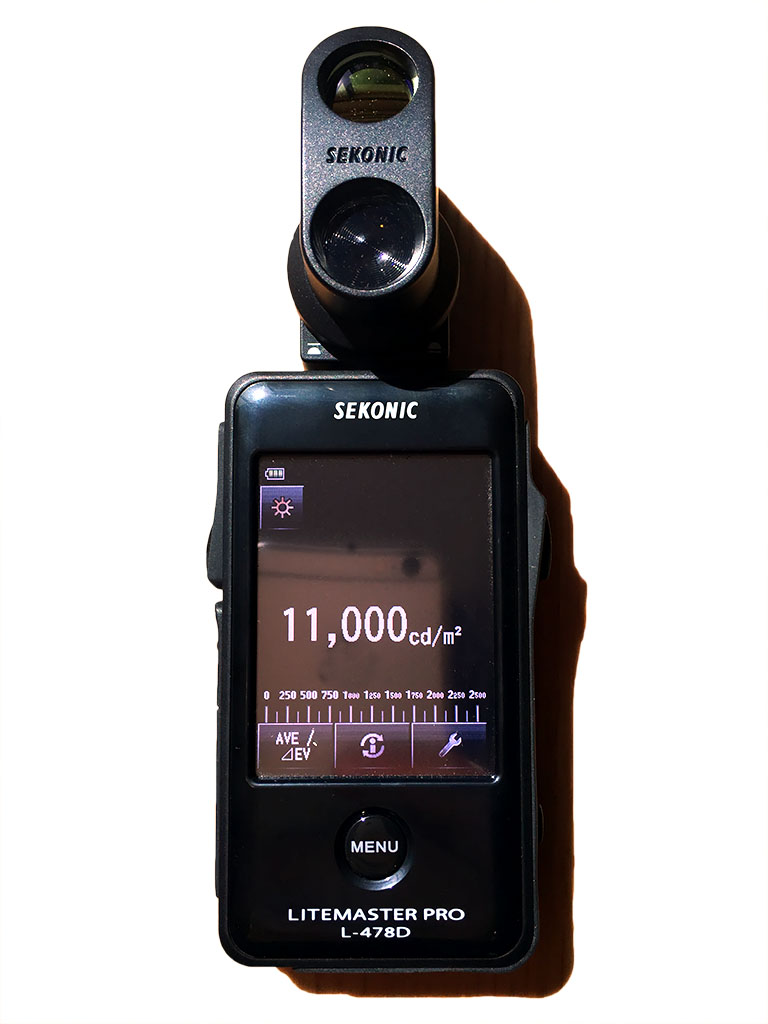
#### Luminous intensity
The luminous intensity of a light source cannot be measured directly but can be derived from the measured illuminance if we know the distance between the measuring device and the light source. Equation $\ref{derivedLuminousIntensity}$ is a simple application of the inverse square law discussed in section [Punctual lights].
$$\begin{equation}\label{derivedLuminousIntensity}
I = E \cdot d^2
\end{equation}$$
## Direct lighting
We have defined the light units for all the light types supported by the renderer in the section above but we have not defined the light unit for the result of the lighting equations. Choosing physical light units means that we will compute luminance values in our shaders, and therefore that all our light evaluation functions will compute the luminance $L_{out}$ (or outgoing radiance) at any given point. The luminance depends on the illuminance $E$ and the BSDF $f(v,l)$ :
$$\begin{equation}\label{luminanceEquation}
L_{out} = f(v,l)E
\end{equation}$$
### Directional lights
The main purpose of directional lights is to recreate important light sources for outdoor environment, i.e. the sun and/or the moon. While directional lights do not truly exist in the physical world, any light source sufficiently far from the light receptor can be assumed to be directional (i.e. all the incident light rays are parallel, as shown in figure [directionalLight]).
![Figure [directionalLight]: Interaction between a directional light and a surface. The light source is a virtual construct that can only be represented by a direction](images/diagram_directional_light.png)
This approximation proves to work incredibly well for the diffuse response of a surface but the specular response is incorrect. The Frostbite engine solves this problem by treating the "sun" directional light as a disc area light. However, our tests have shown that the quality increase does not justify the added computational costs.
We earlier stated that we chose an illuminance light unit ($lx$) for directional lights. This is in part due to the fact that we can easily find illuminance values for the sky and the sun (online or with a light meter) but also to simplify the luminance equation described in $\ref{luminanceEquation}$.
$$\begin{equation}\label{directionalLuminanceEquation}
L_{out} = f(v,l) E_{\bot} \left< \NoL \right>
\end{equation}$$
In the simplified luminance equation $\ref{directionalLuminanceEquation}$, $E_{\bot}$ is the illuminance of the light source for a surface perpendicular to said light source. If the directional light source simulates the sun, $E_{\bot}$ is the illuminance of the sun for a surface perpendicular to the sun direction.
Table [sunSkyIlluminance] provides useful reference values for the sun and sky illumination, measured[^illuminanceMeasures] on a clear day in March, in California.
Light | 10am | 12pm | 5:30pm
--------------------------:|---------:|---------:|---------:
$Sky_{\bot} + Sun_{\bot}$ | 120,000 | 130,000 | 90,000
$Sky_{\bot}$ | 20,000 | 25,000 | 9,000
$Sun_{\bot}$ | 100,000 | 105,000 | 81,000
[Table [sunSkyIlluminance]: Illuminance values in $lx$ (a full moon has an illuminance of 1 $lx$)]
Dynamic directional lights are particularly cheap to evaluate at runtime, as shown in listing [glslDirectionalLight].
~~~~~~~~~~~~~~~~~~~~~~~~~~~~~~~~~~~~~~
vec3 l = normalize(-lightDirection);
float NoL = clamp(dot(n, l), 0.0, 1.0);
// lightIntensity is the illuminance
// at perpendicular incidence in lux
float illuminance = lightIntensity * NoL;
vec3 luminance = BSDF(v, l) * illuminance;
~~~~~~~~~~~~~~~~~~~~~~~~~~~~~~~~~~~~~~
[Listing [glslDirectionalLight]: Implementation of directional lights in GLSL]
Figure [directionalLightTest] shows the effect of lighting a simple scene with a directional light setup to approximate a midday Sun (illuminance set to 110,000 $lx$). For illustration purposes, only direct lighting is shown.
![Figure [directionalLightTest]: Series of dielectric materials of varying roughness under a directional light](images/screenshot_directional_light.png)
[^illuminanceMeasures]: Measurements taken with an incident light meter (Sekonic L-478D)
### Punctual lights
Our engine will support two types of punctual lights, commonly found in most if not all rendering engines: point lights and spot lights. These types of lights are traditionally physically inaccurate for two reasons:
1. They are truly punctual and infinitesimally small.
2. They do not follow the [inverse square law](http://en.wikipedia.org/wiki/Inverse-square_law).
The first issue can be addressed with area lights but, given the cheaper nature of punctual lights it is deemed practical to use infinitesimally small punctual lights whenever possible.
The second issue is easy to fix. For a given punctual light, the perceived intensity decreases proportionally to the square of the distance from the viewer (more precisely, the light receptor).
For punctual lights following the inverse square law, the term $E$ of equation $ \ref{luminanceEquation} $ is expressed in equation $\ref{punctualLightEquation}$, where $d$ is the distance from a point at the surface to the light.
$$\begin{equation}\label{punctualLightEquation}
E = L_{in} \left< \NoL \right> = \frac{I}{d^2} \left< \NoL \right>
\end{equation}$$
The difference between point and spot lights lies in how $E$ is computed, and in particular how the luminous intensity $I$ is computed from the luminous power $\Phi$.
#### Point lights
A point light is defined only by a position in space, as shown in figure [pointLight].
![Figure [pointLight]: Interaction between a point light and a surface. The attenuation only depends on the distance to the light](images/diagram_point_light.png)
The luminous power of a point light is calculated by integrating the luminous intensity over the light's solid angle, as show in equation $\ref{pointLightLuminousPower}$. The luminous intensity can then be easily derived from the luminous power.
$$\begin{equation}\label{pointLightLuminousPower}
\Phi = \int_{\Omega} I dl = \int_{0}^{2\pi} \int_{0}^{\pi} I d\theta d\phi = 4 \pi I \\
I = \frac{\Phi}{4 \pi}
\end{equation}$$
By simple substitution of $I$ in $\ref{punctualLightEquation}$ and $E$ in $ \ref{luminanceEquation} $ we can formulate the luminance equation of a point light as a function of the luminous power (see $ \ref{pointLightLuminanceEquation} $).
$$\begin{equation}\label{pointLightLuminanceEquation}
L_{out} = f(v,l) \frac{\Phi}{4 \pi d^2} \left< \NoL \right>
\end{equation}$$
Figure [pointLightTest] shows the effect of lighting a simple scene with a point light subject to distance attenuation. Light falloff is exaggerated for illustration purposes.
![Figure [pointLightTest]: Inverse square law applied to point lights evaluation](images/screenshot_point_light.png)
#### Spot lights
A spot light is defined by a position in space, a direction vector and two cone angles, $ \theta_{inner} $ and $ \theta_{outer} $ (see figure [spotLight]). These two angles are used to define the angular falloff attenuation of the spot light. The light evaluation function of a spot light must therefore take into account both the inverse square law and these two angles to properly evaluate the luminance attenuation.
![Figure [spotLight]: Interaction between a spot light and a surface. The attenuation depends on the distance to the light and the angle between the surface the spot light's direction vector](images/diagram_spot_light.png)
Equation $ \ref{spotLightLuminousPower} $ describes how the luminous power of a spot light can be calculated in a similar fashion to point lights, using $ \theta_{outer} $ the outer angle of the spot light's cone in the range [0..$\pi$].
$$\begin{equation}\label{spotLightLuminousPower}
\Phi = \int_{\Omega} I dl = \int_{0}^{2\pi} \int_{0}^{\theta_{outer}} I d\theta d\phi = 2 \pi (1 - cos\frac{\theta_{outer}}{2})I \\
I = \frac{\Phi}{2 \pi (1 - cos\frac{\theta_{outer}}{2})}
\end{equation}$$
While this formulation is physically correct, it makes spot lights a little difficult to use: changing the outer angle of the cone changes the illumination levels. Figure [spotLightTestFocused] shows the same scene lit by a spot light, with an outer angle of 55 degrees and an outer angle of 15 degrees. Observes how the illumination level increases as the cone aperture decreases.
![Figure [spotLightTestFocused]: Comparison of spot light outer angles, 55 degrees (left) and 15 degrees (right)](images/screenshot_spot_light_focused.png)
The coupling of illumination and the outer cone means that an artist cannot tweak the influence cone of a spot light without also changing the perceived illumination. It therefore makes sense to provide artists with a parameter to disable this coupling. Equations $ \ref{spotLightLuminousPowerB} $ shows how to formulate the luminous power for that purpose.
$$\begin{equation}\label{spotLightLuminousPowerB}
\Phi = \pi I \\
I = \frac{\Phi}{\pi} \\
\end{equation}$$
With this new formulation to compute the luminous intensity, the test scene in figure [spotLightTest] exhibits similar illumination levels with both cone apertures.
![Figure [spotLightTest]: Comparison of spot light outer angles, 55 degrees (left) and 15 degrees (right)](images/screenshot_spot_light.png)
This new formulation can also be considered physically based if the spot's reflector is replaced with a matte, diffuse mask that absorbs light perfectly.
The spot light evaluation function can be expressed in two ways:
- **With a light absorber**
$$\begin{equation}\label{spotAbsorber}
L_{out} = f(v,l) \frac{\Phi}{\pi d^2} \left< \NoL \right> \lambda(l)
\end{equation}$$
- **With a light reflector**
$$\begin{equation}\label{spotReflector}
L_{out} = f(v,l) \frac{\Phi}{2 \pi (1 - cos\frac{\theta_{outer}}{2}) d^2} \left< \NoL \right> \lambda(l)
\end{equation}$$
The term $ \lambda(l) $ in equations $ \ref{spotAbsorber} $ and $ \ref{spotReflector} $ is the spot's angle attenuation factor described in equation
$ \ref{spotAngleAtt} $ below.
$$\begin{equation}\label{spotAngleAtt}
\lambda(l) = \frac{l \cdot spotDirection - cos\theta_{outer}}{cos\theta_{inner} - cos\theta_{outer}}
\end{equation}$$
#### Attenuation function
A proper evaluation of the inverse square law attenuation factor is mandatory for physically based punctual lights. The simple mathematical formulation is unfortunately impractical for implementation purposes:
1. The division by the squared distance can lead to divides by 0 when objects intersect or "touch" light sources.
2. The influence sphere of each light is infinite ($ \frac{I}{d^2} $ is asymptotic, it never reaches 0) which means that to correctly shade a pixel we need to evaluate every light in the world.
The first issue can be solved easily by setting the assumption that punctual lights are not truly punctual but instead small area lights. To do this we can simply treat punctual lights as spheres of 1 cm radius, as show in equation $\ref{finitePunctualLight}$.
$$\begin{equation}\label{finitePunctualLight}
E = \frac{I}{max(d^2, {0.01}^2)}
\end{equation}$$
We can solve the second issue by introducing an influence radius for each light. There are several advantages to this solution. Tools can quickly show artists what parts of the world will be influenced by every light (the tool just needs to draw a sphere centered on each light). The rendering engine can cull lights more aggressively using this extra piece of information and artists/developers can assist the engine by manually tweaking the influence radius of a light.
Mathematically, the illuminance of a light should smoothly reach zero at the limit defined by the influence radius. [#Karis13b] proposes to window the inverse square function in such a way that the majority of the light's influence remains unaffected. The proposed windowing is described in equation $\ref{attenuationWindowing}$, where $r$ is the light's radius of influence.
$$\begin{equation}\label{attenuationWindowing}
E = \frac{I}{max(d^2, {0.01}^2)} \left< 1 - \frac{d^4}{r^4} \right>^2
\end{equation}$$
Listing [glslPunctualLight] demonstrates how to implement physically based punctual lights in GLSL. Note that the light intensity used in this piece of code is the luminous intensity $I$ in $cd$, converted from the luminous power CPU-side. This snippet is not optimized and some of the computations can be offloaded to the CPU (for instance the square of the light's inverse falloff radius, or the spot scale and angle).
~~~~~~~~~~~~~~~~~~~~~~~~~~~~~~~~~~~~~~
float getSquareFalloffAttenuation(vec3 posToLight, float lightInvRadius) {
float distanceSquare = dot(posToLight, posToLight);
float factor = distanceSquare * lightInvRadius * lightInvRadius;
float smoothFactor = max(1.0 - factor * factor, 0.0);
return (smoothFactor * smoothFactor) / max(distanceSquare, 1e-4);
}
float getSpotAngleAttenuation(vec3 l, vec3 lightDir,
float innerAngle, float outerAngle) {
// the scale and offset computations can be done CPU-side
float cosOuter = cos(outerAngle);
float spotScale = 1.0 / max(cos(innerAngle) - cosOuter, 1e-4)
float spotOffset = -cosOuter * spotScale
float cd = dot(normalize(-lightDir), l);
float attenuation = clamp(cd * spotScale + spotOffset, 0.0, 1.0);
return attenuation * attenuation;
}
vec3 evaluatePunctualLight() {
vec3 l = normalize(posToLight);
float NoL = clamp(dot(n, l), 0.0, 1.0);
vec3 posToLight = lightPosition - worldPosition;
float attenuation;
attenuation = getSquareFalloffAttenuation(posToLight, lightInvRadius);
attenuation *= getSpotAngleAttenuation(l, lightDir, innerAngle, outerAngle);
vec3 luminance = (BSDF(v, l) * lightIntensity * attenuation * NoL) * lightColor;
return luminance;
}
~~~~~~~~~~~~~~~~~~~~~~~~~~~~~~~~~~~~~~
[Listing [glslPunctualLight]: Implementation of punctual lights in GLSL]
### Photometric lights
Punctual lights are an extremely practical and efficient way to light a scene but do not give artists enough control over the light distribution. The field of architectural lighting design concerns itself with designing lighting systems to serve humans needs by taking into account:
- The amount of light provided
- The color of the light
- The distribution of light within the space
The lighting system we have described so far can easily address the first two points but we need a way to define the distribution of light within the space. Light distribution is especially important for indoor scenes or for some types of outdoor scenes or even road lighting. Figure [lightDistributionTest] shows scenes where the light distribution is controlled by the artist. This type of distribution control is widely used when putting objects on display (museums, stores or galleries for instance).
![Figure [lightDistributionTest]: Controlling the distribution of a point light](images/screenshot_photometric_lights.png)
Photometric lights use a photometric profile to describe their intensity distribution. There are two commonly used formats, IES (Illuminating Engineering Society) and EULUMDAT (European Lumen Data format) but we will focus on the former. IES profiles are supported by many tools and engines, such as Unreal Engine 4, Frostbite, Renderman, Maya and Killzone. In addition, IES light profiles are commonly made available by bulbs and luminaires manufacturers (Philips offers [an extensive array of IES files](http://www.usa.lighting.philips.com/connect/tools_literature/photometric_data_1.wpd) for download for instance). Photometric profiles are particularly useful when they measure a luminaire or light fixture, in which the light source is partially covered. The luminaire will block the light emitted in certain directions, thus shaping the light distribution.
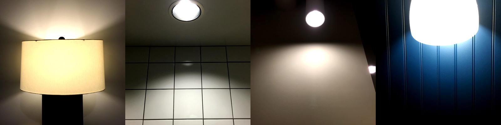
An IES profile stores luminous intensity for various angles on a sphere around the measured light source. This spherical coordinate system is usually referred to as the photometric web, which can be visualized using specialized tools such as [IESviewer](http://www.photometricviewer.com/). Figure [xarrow] below shows the photometric web of the XArrow IES profile [provided by Pixar](http://renderman.pixar.com/view/DP25764) for use with Renderman. This picture also shows a rendering in 3D space of the XArrow IES profile by our tool `lightgen`.
![Figure [xarrow]: The XArrow IES profile rendered as a photometric web and as a point light in 3D space](images/screenshot_xarrow.png)
The IES format is poorly documented and it is not uncommon to find syntax variations between files found on the Internet. The best resource to understand IES profile is Ian Ashdown's "Parsing the IESNA LM-63 photometric data file" document [#Ashdown98]. Succinctly, an IES profiles stores luminous intensities in candela at various angles around the light source. For each measured horizontal angle, a series of luminous intensities at different vertical angles is provided. It is however fairly common for measured light sources to be horizontally symmetrical. The XArrow profile shown above is a good example: intensities vary with vertical angles (vertical axis) but are symmetrical on the horizontal axis. The range of vertical angles in an IES profile is 0 to 180 degrees and the range of horizontal angles is 0 to 360 degrees.
Figure [lightenSamples] shows the series of IES profiles provided by Pixar for Renderman, rendered using our `lightgen` tool.
![Figure [lightenSamples]: Series of IES light profiles rendered with lightgen](images/screenshot_lightgen_samples.png)
IES profiles can be applied directly to any punctual light, point or spot. To do so, we must first process the IES profile and generate a photometric profile as a texture. For performance considerations, the photometric profile we generate is a 1D texture that represents the average luminous intensity for all horizontal angles at a specific vertical angle (i.e., each pixel represents a vertical angle). To truly represent a photometric light, we should use a 2D texture but since most lights are fully, or mostly, symmetrical on the horizontal plane, we can accept this approximation. The values stored in the texture are normalized by the inverse maximum intensity defined in the IES profile. This allows us to easily store the texture in any float format or, at the cost of a bit of precision, in a luminance 8-bit texture (grayscale PNG for instance). Storing normalized values also allows us to treat photometric profiles as a mask:
Photometric profile as a mask
: The luminous intensity is defined by the artist by setting the luminous power of the light, as with any other punctual light. The artist defined intensity is divided by the intensity of the light computed from the IES profile. IES profiles contain a luminous intensity but it is only valid for a bare light bulb whereas the measured intensity values take into account the light fixture. To measure the intensity of the luminaire, instead of the bulb, we perform a Monte-Carlo integration of the unit sphere using the intensities from the profile[^xarrowIntensity].
Photometric profile
: The luminous intensity comes from the profile itself. All the values sampled from the 1D texture are simply multiplied by the maximum intensity. We also provide a multiplier for convenience.
The photometric profile can be applied at rendering time as a simple attenuation. The luminance equation $ \ref{photometricLightEvaluation} $ describes the photometric point light evaluation function.
$$\begin{equation}\label{photometricLightEvaluation}
L_{out} = f(v,l) \frac{I}{d^2} \left< \NoL \right> \Psi(l)
\end{equation}$$
The term $ \Psi(l) $ is the photometric attenuation function. It depends on the light vector, but also on the direction of the light. Spot lights already possess a direction vector but we need to introduce one for photometric point lights as well.
The photometric attenuation function can be easily implemented in GLSL by adding a new attenuation factor to the implementation of punctual lights (listing [glslPunctualLight]). The modified implementation is show in listing [glslPhotometricPunctualLight].
~~~~~~~~~~~~~~~~~~~~~~~~~~~~~~~~~~~~~~
float getPhotometricAttenuation(vec3 posToLight, vec3 lightDir) {
float cosTheta = dot(-posToLight, lightDir);
float angle = acos(cosTheta) * (1.0 / PI);
return texture2DLodEXT(lightProfileMap, vec2(angle, 0.0), 0.0).r;
}
vec3 evaluatePunctualLight() {
vec3 l = normalize(posToLight);
float NoL = clamp(dot(n, l), 0.0, 1.0);
vec3 posToLight = lightPosition - worldPosition;
float attenuation;
attenuation = getSquareFalloffAttenuation(posToLight, lightInvRadius);
attenuation *= getSpotAngleAttenuation(l, lightDirection, innerAngle, outerAngle);
attenuation *= getPhotometricAttenuation(l, lightDirection);
float luminance = (BSDF(v, l) * lightIntensity * attenuation * NoL) * lightColor;
return luminance;
}
~~~~~~~~~~~~~~~~~~~~~~~~~~~~~~~~~~~~~~
[Listing [glslPhotometricPunctualLight]: Implementation of attenuation from photometric profiles in GLSL]
The light intensity is computed CPU-side (listing [photometricLightIntensity]) and depends on whether the photometric profile is used as a mask.
~~~~~~~~~~~~~~~~~~~~~~~~~~~~~~~~~~~~~~
float multiplier;
// Photometric profile used as a mask
if (photometricLight.isMasked()) {
// The desired intensity is set by the artist
// The integrated intensity comes from a Monte-Carlo
// integration over the unit sphere around the luminaire
multiplier = photometricLight.getDesiredIntensity() /
photometricLight.getIntegratedIntensity();
} else {
// Multiplier provided for convenience, set to 1.0 by default
multiplier = photometricLight.getMultiplier();
}
// The max intensity in cd comes from the IES profile
float lightIntensity = photometricLight.getMaxIntensity() * multiplier;
~~~~~~~~~~~~~~~~~~~~~~~~~~~~~~~~~~~~~~
[Listing [photometricLightIntensity]: Computing the intensity of a photometric light on the CPU]
[^xarrowIntensity]: The XArrow profile declares a luminous intensity of 1,750 lm but a Monte-Carlo integration shows an intensity of only 350 lm.
### Area lights
[TODO]
### Lights parameterization
Similarly to the parameterization of the standard material model, our goal is to make lights parameterization intuitive and easy to use for artists and developers alike. In that spirit, we decided to separate the light color (or hue) from the light intensity. A light color will therefore be defined as a linear RGB color (or sRGB in the tools UI for convenience).
The full list of light parameters is presented in table [lightParameters].
Parameter | Definition
--------------------------:|:---------------------
**Type** | Directional, point, spot or area
**Direction** | Used for directional lights, spot lights, photometric point lights, and linear and tubular area lights (orientation)
**Color** | The color of emitted light, as a linear RGB color. Can be specified as an sRGB color or a color temperature in the tools
**Intensity** | The light's brightness. The unit depends on the type of light
**Falloff radius** | Maximum distance of influence
**Inner angle** | Angle of the inner cone for spot lights, in degrees
**Outer angle** | Angle of the outer cone for spot lights, in degrees
**Length** | Length of the area light, used to create linear or tubular lights
**Radius** | Radius of the area light, used to create spherical or tubular lights
**Photometric profile** | Texture representing a photometric light profile, works only for punctual lights
**Masked profile** | Boolean indicating whether the IES profile is used as a mask or not. When used as a mask, the light's brightness will be multiplied by the ratio between the user specified intensity and the integrated IES profile intensity. When not used as a mask, the user specified intensity is ignored but the IES multiplier is used instead
**Photometric multiplier** | Brightness multiplier for photometric lights (if IES as mask is turned off)
[Table [lightParameters]: Light types parameters]
**Note**: to simplify the implementation, all luminous powers will converted to luminous intensities ($cd$) before being sent to the shader. The conversion is light dependent and is explained in the previous sections.
**Note**: the light type can be inferred from other parameters (e.g. a point light has a length, radius, inner angle and outer angle of 0).
#### Color temperature
However, real-world artificial lights are often defined by their color temperature, measured in Kelvin (K). The color temperature of a light source is the temperature of an ideal black-body radiator that radiates light of comparable hue to that of the light source. For convenience, the tools should allow the artist to specify the hue of a light source as a color temperature (a meaningful range is 1,000 K to 12,500 K).
To compute RGB values from a temperature, we can use the Planckian locus, shown in figure [planckianLocus]. This locus is the path that the color of an incandescent black body takes in a chromaticity space as the body's temperature changes.
![Figure [planckianLocus]: The Planckian locus visualized on a CIE 1931 chromaticity diagram (source: Wikipedia)](images/diagram_planckian_locus.png)
The easiest way to compute RGB values from this locus is to use the formula described in [#Krystek85]. Krystek's algorithm (equation $\ref{krystek}$) works in the CIE 1960 (UCS) space, using the following formula where $T$ is the desired temperature, and $u$ and $v$ the coordinates in UCS.
$$\begin{equation}\label{krystek}
u(T) = \frac{0.860117757 + 1.54118254 \times 10^{-4}T + 1.28641212 \times 10^{-7}T^2}{1 + 8.42420235 \times 10^{-4}T + 7.08145163 \times 10^{-7}T^2} \\
v(T) = \frac{0.317398726 + 4.22806245
\times 10^{-5}T + 4.20481691 \times 10^{-8}T^2}{1 - 2.89741816
\times 10^{-5}T + 1.61456053 \times 10^{-7}T^2}
\end{equation}$$
This approximation is accurate to roughly $ 9 \times 10^{-5} $ in the range 1,000K to 15,000K. From the CIE 1960 space we can compute the coordinates in xyY space (CIES 1931), using the formula from equation $\ref{cieToxyY}$.
$$\begin{equation}\label{cieToxyY}
x = \frac{3u}{2u - 8v + 4} \\
y = \frac{2v}{2u - 8v + 4}
\end{equation}$$
The formulas above are valid for black body color temperatures, and therefore correlated color temperatures of standard illuminants. If we wish to compute the precise chromaticity coordinates of standard CIE illuminants in the D series we can use equation $\ref{seriesDtoxyY}$.
$$\begin{equation}\label{seriesDtoxyY}
x = \begin{cases} 0.244063 + 0.09911 \frac{10^3}{T} + 2.9678 \frac{10^6}{T^2} - 4.6070 \frac{10^9}{T^3} & 4,000K \le T \le 7,000K \\
0.237040 + 0.24748 \frac{10^3}{T} + 1.9018 \frac{10^6}{T^2} - 2.0064 \frac{10^9}{T^3} & 7,000K \le T \le 25,000K \end{cases} \\
y = -3x^2 + 2.87 x - 0.275
\end{equation}$$
From the xyY space, we can then convert to the CIE XYZ space (equation $\ref{xyYtoXYZ}$).
$$\begin{equation}\label{xyYtoXYZ}
X = \frac{xY}{y} \\
Z = \frac{(1 - x - y)Y}{y}
\end{equation}$$
For our needs, we will fix $Y = 1$. This allows us to convert from the XYZ space to linear RGB with a simple 3x3 matrix, as shown in equation $\ref{XYZtoRGB}$.
$$\begin{equation}\label{XYZtoRGB}
\left[ \begin{matrix} R \\ G \\ B \end{matrix} \right] = M^{-1} \left[ \begin{matrix} X \\ Y \\ Z \end{matrix} \right]
\end{equation}$$
The transformation matrix M is calculated from the target RGB color space primaries. Equation $ \ref{XYZtoRGBValues} $ shows the conversion using the inverse matrix for the sRGB color space.
$$\begin{equation}\label{XYZtoRGBValues}
\left[ \begin{matrix} R \\ G \\ B \end{matrix} \right] = \left[ \begin{matrix} 3.2404542 & -1.5371385 & -0.4985314 \\ -0.9692660 & 1.8760108 & 0.0415560 \\ 0.0556434 & -0.2040259 & 1.0572252 \end{matrix} \right] \left[ \begin{matrix} X \\ Y \\ Z \end{matrix} \right]
\end{equation}$$
The result of these operations is a linear RGB triplet in the sRGB color space. Since we care about the chromaticity of the results, we must apply a normalization step to avoid clamping values greater than 1.0 and distort resulting colors:
$$\begin{equation}\label{normalizedRGB}
\hat{C}_{linear} = \frac{C_{linear}}{max(C_{linear})}
\end{equation}$$
We must finally apply the sRGB opto-electronic conversion function (OECF, shown in equation $ \ref{OECFsRGB} $) to obtain a displayable value (the value should remain linear if passed to the renderer for shading).
$$\begin{equation}\label{OECFsRGB}
C_{sRGB} = \begin{cases} 12.92 \times \hat{C}_{linear} & \hat{C}_{linear} \le 0.0031308 \\
1.055 \times \hat{C}_{linear}^{\frac{1}{2.4}} - 0.055 & \hat{C}_{linear} \gt 0.0031308 \end{cases}
\end{equation}$$
For convenience, figure [colorTemperatureScaleCCT] shows the range of correlated color temperatures from 1,000K to 12,500K. All the colors used below assume CIE $ D_{65} $ as the white point (as is the case in the sRGB color space).
![Figure [colorTemperatureScaleCCT]: Scale of correlated color temperatures](images/diagram_color_temperature_cct.png)
Similarly, figure [colorTemperatureScaleCIE] shows the range of CIE standard illuminants series D from 1,000K to 12,500K.
![Figure [colorTemperatureScaleCIE]: Scale of CIE standard illuminants series D](images/diagram_color_temperature_cie.png)
For reference, figure [colorTemperatureScaleCCTClamped] shows the range of correlated color temperatures without the normalization step presented in equation $\ref{normalizedRGB}$.
![Figure [colorTemperatureScaleCCTClamped]: Unnormalized scale of correlated color temperatures](images/diagram_color_temperature_cct_clamped.png)
Table [colorTemperatureSamples] presents the correlated color temperature of various common light sources as sRGB color swatches. These colors are relative to the $ D_{65} $ white point, so their perceived hue might vary based on your display's white point. See [What colour is the Sun?](http://jila.colorado.edu/~ajsh/colour/Tspectrum.html) for more information.
Temperature (K) | Light source | Color
--------------------:|:-----------------------------|-------------------------------------------------------
1,700-1,800 | Match flame |
1,850-1,930 | Candle flame |
2,000-3,000 | Sun at sunrise/sunset |
2,500-2,900 | Household tungsten lightbulb |
3,000 | Tungsten lamp 1K |
3,200-3,500 | Quartz lights |
3,200-3,700 | Fluorescent lights |
3,275 | Tungsten lamp 2K |
3,380 | Tungsten lamp 5K, 10K |
5,000-5,400 | Sun at noon |
5,500-6,500 | Daylight (sun + sky) |
5,500-6,500 | Sun through clouds/haze |
6,000-7,500 | Overcast sky |
6,500 | RGB monitor white point |
7,000-8,000 | Shaded areas outdoors |
8,000-10,000 | Partly cloudy sky |
[Table [colorTemperatureSamples]: Normalized correlated color temperatures for common light sources]
### Pre-exposed lights
Physically based rendering and physical light units pose an interesting challenge: how to store and handle the large range of values produced by the lighting code? Assuming computations performed at full precision in the shaders, we still want to be able to store the linear output of the lighting pass in a reasonably sized buffer (`RGB16F` or equivalent). The most obvious and easiest way to achieve this is to simply apply the camera exposure (see the Physically based camera section for more information) before writing out the result of the lighting pass. This simple step is shown in listing [preexposedLighting]:
~~~~~~~~~~~~~~~~~~~~~~~~~~~~~~~~~~~~~~
fragColor = luminance * camera.exposure;
~~~~~~~~~~~~~~~~~~~~~~~~~~~~~~~~~~~~~~
[Listing [preexposedLighting]: The output of the lighting pass is pre-exposed to fit in half-float buffers]
This solution solves the storage problem but requires intermediate computations to be performed with single precision floats. We would instead prefer to perform all (or at least most) of the lighting work using half precision floats instead. Doing so can greatly improve performance and power usage, particularly on mobile devices. Half precision floats are however ill-suited for this kind of work as common illuminance and luminance values (for the sun for instance) can exceed their range. The solution is to simply pre-expose the lights themselves instead of the result of the lighting pass. This can be done efficiently on the CPU if updating a light's constant buffer is cheap. This can also be done on the GPU, as shown in listing [preexposedLights].
~~~~~~~~~~~~~~~~~~~~~~~~~~~~~~~~~~~~~~
// The inputs must be highp/single precision,
// both for range (intensity) and precision (exposure)
// The output is mediump/half precision
float computePreExposedIntensity(highp float intensity, highp float exposure) {
return intensity * exposure;
}
Light getPointLight(uint index) {
Light light;
uint lightIndex = // fetch light index;
// the intensity must be highp/single precision
highp vec4 colorIntensity = lightsUniforms.lights[lightIndex][1];
// pre-expose the light
light.colorIntensity.w = computePreExposedIntensity(
colorIntensity.w, frameUniforms.exposure);
return light;
}
~~~~~~~~~~~~~~~~~~~~~~~~~~~~~~~~~~~~~~
[Listing [preexposedLights]: Pre-exposing lights allows the entire shading pipeline to use half precision floats]
In practice we pre-expose the following lights:
- Punctual lights (point and spot): on the GPU
- Directional light: on the CPU
- IBLs: on the CPU
- Material emissive: on the GPU
## Image based lights
In real life, light comes from every direction either directly from light sources or indirectly after bouncing off objects in the environment, being partially absorbed in the process. In a way the whole environment around an object can be seen as a light source. Images, in particular cubemaps, are a great way to encode such an “environment light”. This is called Image Based Lighting (IBL) or sometimes Indirect Lighting.
![Figure [iblBall]: The object shown here is lit only by image-encoded environment lights. Notice the subtle lighting effects that can be applied using this technique.](images/screenshot_ball_ibl.png)
There are limitations with image-based lighting. Obviously the environment image must be acquired somehow and as we'll see below it needs to be pre-processed before it can be used for lighting. Typically, the environment image is acquired offline in the real world, or generated by the engine either offline or at run time; either way, local or distant probes are used.
These probes can be used to acquire the distant or local environment. In this document, we're focusing on distant environment probes, where the light is assumed to come from infinitely far away (which means every point on the object's surface uses the same environment map).
The whole environment contributes light to a given point on the object's surface; this is called _irradiance_ ($E$). The resulting light bouncing off of the object is called radiance ($L_{out}$). Incident lighting must be applied consistently to the diffuse and specular parts of the BRDF.
The radiance $L_{out}$ resulting from the interaction between an image based light's (IBL) irradiance and a material model (BRDF) $f(\Theta)$[^ibl1] is computed as follows:
$$\begin{equation}
L_{out}(n, v, \Theta) = \int_\Omega f(l, v, \Theta) L_{\bot}(l) \left< \NoL \right> dl
\end{equation}$$
Note that here we're looking at the behavior of the surface at **macro** level (not to be confused with the micro level equation), which is why it only depends on $\vec n$ and $\vec v$. Essentially, we're applying the BRDF to “point-lights” coming from all directions and encoded in the IBL.
### IBL Types ###
There are four common types of IBLs used in modern rendering engines:
- **Distant light probes**, used to capture lighting information at "infinity", where parallax can be ignored. Distant probes typically contain the sky, distant landscape features or buildings, etc. They are either captured by the engine or acquired from a camera as high dynamic range images (HDRI).
- **Local light probes**, used to capture a certain area of the world from a specific point of view. The capture is projected on a cube or sphere depending on the surrounding geometry. Local probes are more accurate than distance probes and are particularly useful to add local reflections to materials.
- **Planar reflections**, used to capture reflections by rendering the scene mirrored by a plane. This technique works only for flat surfaces such as building floors, roads and water.
- **Screen space reflection**, used to capture reflections based on the rendered scene (using the previous frame for instance) by ray-marching in the depth buffer. SSR gives great result but can be very expensive.
In addition we must distinguish between static and dynamic IBLs. Implementing a fully dynamic day/night cycle requires for instance to recompute the distant light probes dynamically[^iblTypes1]. Both planar and screen space reflections are inherently dynamic.
### IBL Unit ###
As discussed previously in the direct lighting section, all our lights must use physical units. As such our IBLs will use the luminance unit $\frac{cd}{m^2}$, which is also the output unit of all our direct lighting equations. Using the luminance unit is straightforward for light probes captures by the engine (dynamically or statically offline).
High dynamic range images are a bit more delicate to handle however. Cameras do not record measured luminance but a device-dependent value that is only _related_ to the original scene luminance. As such, we must provide artists with a multiplier that allows them to recover, or at the very least closely approximate, the original absolute luminance.
To properly reconstruct the luminance of an HDRI for IBL, artists must do more than simply take photos of the environment and record extra information:
- **Color calibration**: using a gray card or a [MacBeth ColorChecker](http://en.wikipedia.org/wiki/ColorChecker)
- **Camera settings**: aperture, shutter and ISO
- **Luminance samples**: using a spot/luminance meter
[TODO] Measure and list common luminance values (clear sky, interior, etc.)
### Processing light probes ###
We saw previously that the radiance of an IBL is computed by integrating over the surface's hemisphere. Since this would obviously be too expensive to do in real-time, we must first pre-process our light probes to convert them into a format better suited for real-time interactions.
The sections below will discuss the techniques used to accelerate the evaluation of light probes:
- **Specular reflectance**: pre-filtered importance sampling and split-sum approximation
- **Diffuse reflectance**: irradiance map and spherical harmonics
### Distant light probes ###
#### Diffuse BRDF integration ####
Using the Lambertian BRDF[^iblDiffuse1], we get the radiance:
$$
\begin{align*}
f_d(\sigma) &= \frac{\sigma}{\pi} \\
L_d(n, \sigma) &= \int_{\Omega} f_d(\sigma) L_{\bot}(l) \left< \NoL \right> dl \\
&= \frac{\sigma}{\pi} \int_{\Omega} L_{\bot}(l) \left< \NoL \right> dl \\
&= \frac{\sigma}{\pi} E_d(n) \quad \text{with the irradiance} \;
E_d(n) = \int_{\Omega} L_{\bot}(l) \left< \NoL \right> dl
\end{align*}
$$
Or in the discrete domain:
$$ E_d(n) \equiv \sum_{\forall \, i \in image} L_{\bot}(s_i) \left< n \cdot s_i \right> \Omega_s $$
$\Omega_s$ is the solid-angle[^iblDiffuse2] associated to sample $i$.
The irradiance integral $\Ed$ can be trivially, albeit slowly[^iblDiffuse3], precomputed and stored into a cubemap for efficient access at runtime. Typically, _image_ is a cubemap or an equirectangular image. The term $ \frac{\sigma}{\pi} $ is independent of the IBL and is added at runtime to obtain the _radiance_.
![Figure [iblOriginal]: Image-based environment](images/ibl/ibl_river_roughness_m0.png style="max-width:100%;")
![Figure [iblIrradiance]: Image-based irradiance map using the Lambertian BRDF](images/ibl/ibl_irradiance.png style="max-width:100%;")
[^ibl1]: $\Theta$ represents the parameters of the material model $f$, i.e.: _roughness_, albedo and so on...
[^iblTypes1]: This can be done through blending of static probes or by spreading the workload over time
[^iblDiffuse1]: The Lambertian BRDF doesn't depend on $\vec l$, $\vec v$ or $\theta$, so $L_d(n,v,\theta) \equiv L_d(n,\sigma)$
[^iblDiffuse2]: $\Omega_s$ can be approximated by $\frac{2\pi}{6 \cdot width \cdot height}$ for a cubemap
[^iblDiffuse3]: $O(12\,n^2\,m^2)$, with $n$ and $m$ respectively the dimensions of the environment and the precomputed cubemap
However, the irradiance can also be approximated very closely by a decomposition into Spherical Harmonics (SH, described in more details in the Spherical Harmonics section) and calculated at runtime cheaply. It is usually best to avoid texture fetches on mobile and free-up a texture unit. Even if it is stored into a cubemap, it is orders of magnitude faster to pre-compute the integral using SH decomposition followed by a rendering.
SH decomposition is similar in concept to a Fourier transform, it expresses the signal over an orthonormal base in the frequency domain. The properties that interests us most are:
- Very few coefficients are needed to encode $\cosTheta$
- Convolutions by a kernel that _has a circular symmetry_ are very inexpensive and become products in SH space
In practice only 4 or 9 coefficients (i.e.: 2 or 3 bands) are enough for $\cosTheta$ meaning we don't need more either for $\Lt$.
![Figure [iblSH3]: 3 bands (9 coefficients)](images/ibl/ibl_irradiance_sh3.png style="max-width:100%;")
![Figure [iblSH2]: 2 bands (4 coefficients)](images/ibl/ibl_irradiance_sh2.png style="max-width:100%;")
In practice we pre-convolve $\Lt$ with $\cosTheta$ and pre-scale these coefficients by the basis scaling factors $K_l^m$ so that the reconstruction code is as simple as possible in the shader:
~~~~~~~~~~~~~~~~~~~~~~~~~~~~~~~~~~~~~~
vec3 irradianceSH(vec3 n) {
// uniform vec3 sphericalHarmonics[9]
// We can use only the first 2 bands for better performance
return
sphericalHarmonics[0]
+ sphericalHarmonics[1] * (n.y)
+ sphericalHarmonics[2] * (n.z)
+ sphericalHarmonics[3] * (n.x)
+ sphericalHarmonics[4] * (n.y * n.x)
+ sphericalHarmonics[5] * (n.y * n.z)
+ sphericalHarmonics[6] * (3.0 * n.z * n.z - 1.0)
+ sphericalHarmonics[7] * (n.z * n.x)
+ sphericalHarmonics[8] * (n.x * n.x - n.y * n.y);
}
~~~~~~~~~~~~~~~~~~~~~~~~~~~~~~~~~~~~~~
[Listing [irradianceSH]: GLSL code to reconstruct the irradiance from the pre-scaled SH]
Note that with 2 bands, the computation above becomes a single $4 \times 4$ matrix-by-vector multiply.
Additionally, because of the pre-scaling by $K_l^m$, the SH coefficients can be thought of as colors, in particular `sphericalHarmonics[0]` is directly the average irradiance.
#### Specular BRDF integration ####
As we've seen above, the radiance $\Lout$ resulting from the interaction between an IBL's irradiance and a BRDF is:
$$\begin{equation}\label{specularBRDFIntegration}
\Lout(n, v, \Theta) = \int_\Omega f(l, v, \Theta) \Lt(l) \left< \NoL \right> \partial l
\end{equation}$$
We recognize the convolution of $\Lt$ by $f(l, v, \Theta) \left< \NoL \right>$,
i.e.: the environment is *filtered* using the BRDF as a kernel. Indeed at higher roughness,
specular reflections look more *blurry*.
Plugging the expression of $f$ in equation $\ref{specularBRDFIntegration}$, we obtain:
$$\begin{equation}
\Lout(n,v,\Theta) = \int_\Omega D(l, v, \alpha) F(l, v, f_0, f_{90}) V(l, v, \alpha) \left< \NoL \right> \Lt(l) \partial l
\end{equation}$$
This expression depends on $v$, $\alpha$, $f_0$ and $f_{90}$ inside the integral,
which makes its evaluation extremely costly and unsuitable for real-time on mobile
(even using pre-filtered importance sampling).
##### Simplifying the BRDF integration #####
Since there is no closed-form solution or an easy way to compute the $\Lout$ integral, we use a simplified
equation instead: $\hat{I}$, whereby we assume that $v = n$, that is the view direction $v$ is always
equal to the surface normal $n$. Clearly, this assumption will break all view-dependant effects of
the convolution, such as the increased blur in reflections closer to the viewer
(a.k.a. stretchy reflections).
Such a simplification would also have a severe impact on constant environments, such as the white
furnace, because it would affect the magnitude of the constant (i.e. DC) term of the result. We
can at least correct for that by using a scale factor, $K$, in our simplified integral, which
will make sure the average irradiance stay correct when chosen properly.
- $I$ is our original integral, i.e.: $I(g) = \int_\Omega g(l) \left< \NoL \right> \partial l$
- $\hat{I}$ is the simplified integral where $v = n$
- $K$ is a scale factor that ensures the average irradiance is unchanged by $\hat{I}$
- $\tilde{I}$ is our final approximation of $I$, $\tilde{I} = \hat{I} \times K$
Because $I$ is an integral multiplications can be distributed over it. i.e.: $I(g()f()) = I(g())I(f())$.
Armed with that,
$$\begin{equation}
I( f(\Theta) \Lt ) \approx \tilde{I}( f(\Theta) \Lt ) \\
\tilde{I}( f(\Theta) \Lt ) = K \times \hat{I}( f(\Theta) \Lt ) \\
K = \frac{I(f(\Theta))}{\hat{I}(f(\Theta))}
\end{equation}$$
From the equation above we can see that $\tilde{I}$ is equivalent to $I$ when $\Lt$ is a constant,
and yields the correct result:
$$\begin{align*}
\tilde{I}(f(\Theta)\Lt^{constant}) &= \Lt^{constant} \hat{I}(f(\Theta)) \frac{I(f(\Theta))}{\hat{I}(f(\Theta))} \\
&= \Lt^{constant} I(f(\Theta)) \\
&= I(f(\Theta)\Lt^{constant})
\end{align*}$$
Similarly, we can also demonstrate that the result is correct when $v = n$, since in that case $I = \hat{I}$:
$$\begin{align*}
\tilde{I}(f(\Theta)\Lt) &= I(f(\Theta)\Lt) \frac{I(f(\Theta))}{I(f(\Theta))} \\
&= I(f(\Theta)\Lt)
\end{align*}$$
Finally, we can show that the scale factor $K$ satisfies our average irradiance ($\bar{\Lt}$)
requirement by plugging $\Lt = \bar{\Lt} + (\Lt - \bar{\Lt}) = \bar{\Lt} + \Delta\Lt$ into $\tilde{I}$:
$$\begin{align*}
\tilde{I}(f(\Theta)\Lt) &= \tilde{I}\left[f\left(\Theta\right) \left(\bar{\Lt} + \Delta\Lt\right)\right] \\
&= K \times \hat{I}\left[f\left(\Theta\right) \left(\bar{\Lt} + \Delta\Lt\right)\right] \\
&= K \times \left[\hat{I}\left(f\left(\Theta\right)\bar{\Lt}\right) + \hat{I}\left(f\left(\Theta\right)\Delta\Lt\right)\right] \\
&= K \times \hat{I}\left(f\left(\Theta\right)\bar{\Lt}\right) + K \times \hat{I}\left(f\left(\Theta\right) \Delta\Lt\right) \\
&= \tilde{I}\left(f\left(\Theta\right)\bar{\Lt}\right) + \tilde{I}\left(f\left(\Theta\right) \Delta\Lt\right) \\
&= I\left(f\left(\Theta\right)\bar{\Lt}\right) + \tilde{I}\left(f\left(\Theta\right) \Delta\Lt\right)
\end{align*}$$
The above result shows that the average irradiance is computed correctly, i.e.: $I(f(\Theta)\bar{\Lt})$.
A way to think about this approximation is that it splits the radiance $\Lt$ in two parts,
the average $\bar{\Lt}$ and the delta from the average $\Delta\Lt$ and computes the correct
integration of the average part then adds the simplified integration of the delta part:
$$\begin{equation}
approximation(\Lt) = correct(\bar{\Lt}) + simplified(\Lt - \bar{\Lt})
\end{equation}$$
Now, let's look at each term:
$$\begin{equation}\label{iblPartialEquations}
\hat{I}(f(n, \alpha) \Lt) = \int_\Omega f(l, n, \alpha) \Lt(l) \left< \NoL \right> \partial l \\
\hat{I}(f(n, \alpha)) = \int_\Omega f(l, n, \alpha) \left< \NoL \right> \partial l \\
I(f(n, v, \alpha)) = \int_\Omega f(l, n, v, \alpha) \left< \NoL \right> \partial l
\end{equation}$$
All three of these equations can be easily pre-calculated and stored in look-up tables, as explained
below.
##### Discrete Domain #####
In the discrete domain the equations in \ref{iblPartialEquations} become:
$$\begin{equation}
\hat{I}(f(n, \alpha) \Lt) \equiv \frac{1}{N}\sum_{\forall \, i \in image} f(l_i, n, \alpha) \Lt(l_i) \left<\NoL\right> \\
\hat{I}(f(n, \alpha)) \equiv \frac{1}{N}\sum_{\forall \, i \in image} f(l_i, n, \alpha) \left<\NoL\right> \\
I(f(n, v, \alpha)) \equiv \frac{1}{N}\sum_{\forall \, i \in image} f(l_i, n, v, \alpha) \left<\NoL\right>
\end{equation}$$
However, in practice we're using _importance sampling_ which needs to take the $pdf$ of the distribution
into account and adds a term $\frac{4\left<\VoH\right>}{D(h_i, \alpha)\left<\NoH\right>}$.
See Importance Sampling For The IBL section:
$$\begin{equation}\label{iblImportanceSampling}
\hat{I}(f(n, \alpha) \Lt) \equiv \frac{4}{N}\sum_i^N f(l_i, n, \alpha) \frac{\left<\VoH\right>}{D(h_i, \alpha)\left<\NoH\right>} \Lt(l_i) \left<\NoL\right> \\
\hat{I}(f(n, \alpha)) \equiv \frac{4}{N}\sum_i^N f(l_i, n, \alpha) \frac{\left<\VoH\right>}{D(h_i, \alpha)\left<\NoH\right>} \left<\NoL\right> \\
I(f(n, v, \alpha)) \equiv \frac{4}{N}\sum_i^N f(l_i, n, v, \alpha) \frac{\left<\VoH\right>}{D(h_i, \alpha)\left<\NoH\right>} \left<\NoL\right>
\end{equation}$$
Recalling that for $\hat{I}$, we assume that $v = n$, equations \ref{iblImportanceSampling},
simplifies to:
$$\begin{equation}
\hat{I}(f(n, \alpha) \Lt) \equiv \frac{4}{N}\sum_i^N \frac{f(l_i, n, \alpha)}{D(h_i, \alpha)} \Lt(l_i) \left<\NoL\right> \\
\hat{I}(f(n, \alpha)) \equiv \frac{4}{N}\sum_i^N \frac{f(l_i, n, \alpha)}{D(h_i, \alpha)} \left<\NoL\right> \\
I(f(n, v, \alpha)) \equiv \frac{4}{N}\sum_i^N \frac{f(l_i, n, v, \alpha)}{D(h_i, \alpha)} \frac{\left<\VoH\right>}{\left<\NoH\right>} \left<\NoL\right>
\end{equation}$$
Then, the first two equations can be merged together such that $LD(n, \alpha) = \frac{\hat{I}(f(n, \alpha) \Lt)}{\hat{I}(f(n, \alpha))}$
$$\begin{equation}\label{iblLD}
LD(n, \alpha) \equiv \frac{\sum_i^N \frac{f(l_i, n, \alpha)}{D(h_i, \alpha)} \Lt(l_i) \left<\NoL\right>}{\sum_i^N \frac{f(l_i, n, \alpha)}{D(h_i, \alpha)}\left<\NoL\right>}
\end{equation}$$
$$\begin{equation}\label{iblDFV}
I(f(n, v, \alpha)) \equiv \frac{4}{N}\sum_i^N \frac{f(l_i, n, v, \alpha)}{D(h_i, \alpha)} \frac{\left<\VoH\right>}{\left<\NoH\right>} \left<\NoL\right>
\end{equation}$$
Note that at this point, we could almost compute both remaining equations off-line. The only difficulty
is that we don't know $f_0$ nor $f_{90}$ when we precompute those integrals. We will see below that
we can incorporate these terms at runtime for equation \ref{iblDFV}, alas, this is not possible for
equation \ref{iblLD} and we have to assume $f_0 = f_{90} = 1$ (i.e.: the fresnel term always evaluates to 1).
We also have to deal with the visibility term of the brdf, in practice keeping it yields to slightly
worst results compared to the ground truth, so we also set $V = 1$.
Let's substitute $f$ in equations \ref{iblLD} and \ref{iblDFV}:
$$\begin{equation}
f(l_i, n, \alpha) = D(h_i, \alpha)F(f_0, f_{90}, \left<\VoH\right>)V(l_i, v, \alpha)
\end{equation}$$
The first simplification is that the term $D(h_i, \alpha)$ in the brdf cancels out with the
denominator (which came from the $pdf$ due to importance sampling) and F and V disappear since we
assume their value is 1.
$$\begin{equation}
LD(n, \alpha) \equiv \frac{\sum_i^N V(l_i, v, \alpha)\left<\NoL\right>\Lt(l_i) }{\sum_i^N \left<\NoL\right>}
\end{equation}$$
$$\begin{equation}\label{iblFV}
I(f(n, v, \alpha)) \equiv \frac{4}{N}\sum_i^N \color{green}{F(f_0, f_{90}, \left<\VoH\right>)} V(l_i, v, \alpha)\frac{\left<\VoH\right>}{\left<\NoH\right>} \left<\NoL\right>
\end{equation}$$
Now, let's substitute the fresnel term into equation \ref{iblFV}:
$$\begin{equation}
F(f_0, f_{90}, \left<\VoH\right>) = f_0 (1 - F_c(\left<\VoH\right>)) + f_{90} F_c(\left<\VoH\right>) \\
F_c(\left<\VoH\right>) = (1 - \left<\VoH\right>)^5
\end{equation}$$
$$\begin{equation}
I(f(n, v, \alpha)) \equiv \frac{4}{N}\sum_i^N \left[\color{green}{f_0 (1 - F_c(\left<\VoH\right>)) + f_{90} F_c(\left<\VoH\right>)}\right] V(l_i, v, \alpha)\frac{\left<\VoH\right>}{\left<\NoH\right>} \left<\NoL\right> \\
\end{equation}$$
$$
\begin{align*}
I(f(n, v, \alpha)) \equiv & \color{green}{f_0 } \frac{4}{N}\sum_i^N \color{green}{(1 - F_c(\left<\VoH\right>))} V(l_i, v, \alpha)\frac{\left<\VoH\right>}{\left<\NoH\right>} \left<\NoL\right> \\
+ & \color{green}{f_{90}} \frac{4}{N}\sum_i^N \color{green}{ F_c(\left<\VoH\right>) } V(l_i, v, \alpha)\frac{\left<\VoH\right>}{\left<\NoH\right>} \left<\NoL\right>
\end{align*}
$$
And finally, we extract the equations that can be calculated off-line (i.e.: the part that doesn't
depend on the runtime parameters $f_0$ and $f_{90}$):
$$\begin{equation}\label{iblAllEquations}
DFG_1(\alpha, \left<\NoV\right>) = \frac{4}{N}\sum_i^N \color{green}{(1 - F_c(\left<\VoH\right>))} V(l_i, v, \alpha)\frac{\left<\VoH\right>}{\left<\NoH\right>} \left<\NoL\right> \\
DFG_2(\alpha, \left<\NoV\right>) = \frac{4}{N}\sum_i^N \color{green}{ F_c(\left<\VoH\right>) } V(l_i, v, \alpha)\frac{\left<\VoH\right>}{\left<\NoH\right>} \left<\NoL\right> \\
I(f(n, v, \alpha)) \equiv \color{green}{f_0} \color{red}{DFG_1(\alpha, \left<\NoV\right>)} + \color{green}{f_{90}} \color{red}{DFG_2(\alpha, \left<\NoV\right>)}
\end{equation}$$
Notice that $DFG_1$ and $DFG_2$ only depend on $\NoV$, that is the angle between the normal $n$ and
the view direction $v$. This is true because the integral is symmetrical with respect to $n$.
When integrating, we can choose any $v$ we please as long as it satisfies $\NoV$
(e.g.: when calculating $\VoH$).
Putting everything back together:
$$
\begin{align*}
\Lout(n,v,\alpha,f_0,f_{90}) &\simeq \big[ f_0 \color{red}{DFG_1(\NoV, \alpha)} + f_{90} \color{red}{DFG_2(\NoV, \alpha)} \big] \times LD(n, \alpha) \\
DFG_1(\alpha, \left<\NoV\right>) &= \frac{4}{N}\sum_i^N \color{green}{(1 - F_c(\left<\VoH\right>))} V(l_i, v, \alpha)\frac{\left<\VoH\right>}{\left<\NoH\right>} \left<\NoL\right> \\
DFG_2(\alpha, \left<\NoV\right>) &= \frac{4}{N}\sum_i^N \color{green}{ F_c(\left<\VoH\right>) } V(l_i, v, \alpha)\frac{\left<\VoH\right>}{\left<\NoH\right>} \left<\NoL\right> \\
LD(n, \alpha) &= \frac{\sum_i^N V(l_i, n, \alpha)\left<\NoL\right>\Lt(l_i) }{\sum_i^N \left<\NoL\right>}
\end{align*}
$$
#### The $DFG_1$ and $DFG_2$ term visualized ####
Both $DFG_1$ and $DFG_2$ can either be pre-calculated in a regular 2D texture indexed by $(\NoV, \alpha)$
and sampled bilinearly, or computed at runtime using an analytic approximation of the surfaces.
See sample code in the annex.
The pre-calculated textures are shown in table [textureDFG].
A C++ implementation of the pre-computation can be found in section [Precomputing L for image-based lighting].
$DFG_1$ | $DFG_2$ | ${ DFG_1, DFG_2, 0 }$
-------------------------|--------------------------|----------------------
 |  | 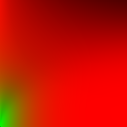
[Table [textureDFG]: Y axis: $\alpha$. X axis: $cos \theta$]
$DFG_1$ and $DFG_2$ are conveniently within the $[0, 1]$ range, however 8-bits textures don't have
enough precision and will cause problems.
Unfortunately, on mobile, 16-bits or float textures are not ubiquitous and there are a limited
number of samplers.
Despite the attractive simplicity of the shader code using a texture, it might be better to use an
analytic approximation. Note however that since we only need to store two terms,
OpenGL ES 3.0's RG16F texture format is a good candidate.
Such analytic approximation is described in [#Karis14], itself based on [#Lazarov13].
[#Narkowicz14] is another interesting approximation. Note that these two approximations are not
compatible with the energy compensation term presented in section [Pre-integration for multiscattering].
Table [textureApproxDFG] presents a visual representation of these approximations.
$DFG_1$ | $DFG_2$ | ${ DFG_1, DFG_2, 0 }$
--------------------------------|---------------------------------|----------------------
 |  | 
[Table [textureApproxDFG]: Y axis: $\alpha$. X axis: $cos \theta$]
#### The $LD$ term visualized ####
$LD$ is the convolution of the environment by a function that only depends on the $\alpha$ parameter
(itself related to the roughness, see section [Roughness remapping and clamping]).
$LD$ can conveniently be stored in a mip-mapped cubemap where increasing LODs receive the environment
pre-filtered with increasing roughness. This works well because this convolution is a
powerful low-pass filter. To make good use of each mipmap level, it is necessary to remap
$\alpha$; we find that using a power remapping with $\gamma = 2$ works well and is convenient.
$$
\begin{align*}
\alpha &= perceptualRoughness^2 \\
lod_{\alpha} &= \alpha^{\frac{1}{2}} = perceptualRoughness \\
\end{align*}
$$
See an example below:


#### Indirect specular and indirect diffuse components visualized ####
Figure [iblVisualized] shows how indirect lighting interacts with dielectrics and conductors. Direct lighting was removed for illustration purposes.
![Figure [iblVisualized]: Indirect diffuse and specular decomposition](images/ibl/ibl_visualization.jpg)
#### IBL evaluation implementation ####
Listing [iblEvaluation] presents a GLSL implementation to evaluate the IBL, using the various textures described in the previous sections.
~~~~~~~~~~~~~~~~~~~~~~~~~~~~~~~~~~~~~~
vec3 ibl(vec3 n, vec3 v, vec3 diffuseColor, vec3 f0, vec3 f90,
float perceptualRoughness) {
vec3 r = reflect(n);
vec3 Ld = textureCube(irradianceEnvMap, r) * diffuseColor;
float lod = computeLODFromRoughness(perceptualRoughness);
vec3 Lld = textureCube(prefilteredEnvMap, r, lod);
vec2 Ldfg = textureLod(dfgLut, vec2(dot(n, v), perceptualRoughness), 0.0).xy;
vec3 Lr = (f0 * Ldfg.x + f90 * Ldfg.y) * Lld;
return Ld + Lr;
}
~~~~~~~~~~~~~~~~~~~~~~~~~~~~~~~~~~~~~~
[Listing [iblEvaluation]: GLSL implementation of image based lighting evaluation]
We can however save a couple of texture lookups by using Spherical Harmonics instead of an
irradiance cubemap and the analytical approximation of the $DFG$ LUT, as shown in listing [optimizedIblEvaluation].
~~~~~~~~~~~~~~~~~~~~~~~~~~~~~~~~~~~~~~
vec3 irradianceSH(vec3 n) {
// uniform vec3 sphericalHarmonics[9]
// We can use only the first 2 bands for better performance
return
sphericalHarmonics[0]
+ sphericalHarmonics[1] * (n.y)
+ sphericalHarmonics[2] * (n.z)
+ sphericalHarmonics[3] * (n.x)
+ sphericalHarmonics[4] * (n.y * n.x)
+ sphericalHarmonics[5] * (n.y * n.z)
+ sphericalHarmonics[6] * (3.0 * n.z * n.z - 1.0)
+ sphericalHarmonics[7] * (n.z * n.x)
+ sphericalHarmonics[8] * (n.x * n.x - n.y * n.y);
}
// NOTE: this is the DFG LUT implementation of the function above
vec2 prefilteredDFG_LUT(float coord, float NoV) {
// coord = sqrt(roughness), which is the mapping used by the
// IBL prefiltering code when computing the mipmaps
return textureLod(dfgLut, vec2(NoV, coord), 0.0).rg;
}
vec3 evaluateSpecularIBL(vec3 r, float perceptualRoughness) {
// This assumes a 256x256 cubemap, with 9 mip levels
float lod = 8.0 * perceptualRoughness;
// decodeEnvironmentMap() either decodes RGBM or is a no-op if the
// cubemap is stored in a float texture
return decodeEnvironmentMap(textureCubeLodEXT(environmentMap, r, lod));
}
vec3 evaluateIBL(vec3 n, vec3 v, vec3 diffuseColor, vec3 f0, vec3 f90, float perceptualRoughness) {
float NoV = max(dot(n, v), 0.0);
vec3 r = reflect(-v, n);
// Specular indirect
vec3 indirectSpecular = evaluateSpecularIBL(r, perceptualRoughness);
vec2 env = prefilteredDFG_LUT(perceptualRoughness, NoV);
vec3 specularColor = f0 * env.x + f90 * env.y;
// Diffuse indirect
// We multiply by the Lambertian BRDF to compute radiance from irradiance
// With the Disney BRDF we would have to remove the Fresnel term that
// depends on NoL (it would be rolled into the SH). The Lambertian BRDF
// can be baked directly in the SH to save a multiplication here
vec3 indirectDiffuse = max(irradianceSH(n), 0.0) * Fd_Lambert();
// Indirect contribution
return diffuseColor * indirectDiffuse + indirectSpecular * specularColor;
}
~~~~~~~~~~~~~~~~~~~~~~~~~~~~~~~~~~~~~~
[Listing [optimizedIblEvaluation]: GLSL implementation of image based lighting evaluation]
#### Pre-integration for multiscattering ####
In section [Energy loss in specular reflectance] we discussed how to use a second scaled specular lobe
to compensate for the energy loss due to only accounting for a single scattering event in our BRDF.
This energy compensation lobe is scaled by a term that depends on $r$ defined in the following way:
$$\begin{equation}
r = \int_{\Omega} D(l,v) V(l,v) \left< \NoL \right> \partial l
\end{equation}$$
Or, evaluated with importance sampling (See Importance Sampling For The IBL section):
$$\begin{equation}
r \equiv \frac{4}{N}\sum_i^N V(l_i, v, \alpha)\frac{\left<\VoH\right>}{\left<\NoH\right>} \left<\NoL\right>
\end{equation}$$
This equality is very similar to the terms $DFG_1$ and $DFG_2$ seen in equation $\ref{iblAllEquations}$.
In fact, it's the same, except without the Fresnel term.
By making the further assumption that $f_{90} = 1$, we can rewrite $DFG_1$ and $DFG_2$ and the
$\Lout$ reconstruction:
$$
\begin{align*}
\Lout(n,v,\alpha,f_0) &\simeq \big[ (1 - f_0) \color{red}{DFG_1^{multiscatter}(\NoV, \alpha)} + f_0 \color{red}{DFG_2^{multiscatter}(\NoV, \alpha)} \big] \times LD(n, \alpha) \\
DFG_1^{multiscatter}(\alpha, \left<\NoV\right>) &= \frac{4}{N}\sum_i^N \color{green}{F_c(\left<\VoH\right>)} V(l_i, v, \alpha)\frac{\left<\VoH\right>}{\left<\NoH\right>} \left<\NoL\right> \\
DFG_2^{multiscatter}(\alpha, \left<\NoV\right>) &= \frac{4}{N}\sum_i^N V(l_i, v, \alpha)\frac{\left<\VoH\right>}{\left<\NoH\right>} \left<\NoL\right> \\
LD(n, \alpha) &= \frac{\sum_i^N V(l_i, n, \alpha)\left<\NoL\right>\Lt(l_i) }{\sum_i^N V(l_i, n, \alpha)\left<\NoL\right>}
\end{align*}
$$
These two new $DFG$ terms simply need to replace the ones used in the implementation shown in section [Precomputing L for image-based lighting]:
~~~~~~~~~~~~~~~~~~~~~~~~~~~~~~~~~~~~~~
float Fc = pow(1 - VoH, 5.0f);
r.x += Gv * Fc;
r.y += Gv;
~~~~~~~~~~~~~~~~~~~~~~~~~~~~~~~~~~~~~~
[Listing [multiscatterIBLPreintegration]: C++ implementation of the $L_{DFG}$ term for multiscattering]
To perform the reconstruction we need to slightly modify listing [multiscatterIBLEvaluation]:
~~~~~~~~~~~~~~~~~~~~~~~~~~~~~~~~~~~~~~
vec2 dfg = textureLod(dfgLut, vec2(dot(n, v), perceptualRoughness), 0.0).xy;
// (1 - f0) * dfg.x + f0 * dfg.y
vec3 specularColor = mix(dfg.xxx, dfg.yyy, f0);
~~~~~~~~~~~~~~~~~~~~~~~~~~~~~~~~~~~~~~
[Listing [multiscatterIBLEvaluation]: GLSL implementation of image based lighting evaluation, with multiscattering LUT]
#### Summary ####
In order to calculate the specular contribution of distant image-based lights, we had to make a few
approximations and compromises:
- $v = n$, by far the assumption contributing to the largest error when integrating the
non-constant part of the IBL. This results in the complete loss of roughness anisotropy
with respect to the view point.
- Roughness contribution for the non-constant part of the IBL is quantized and trilinear filtering
is used to interpolate between these levels. This is most visible at low roughnes (e.g.: around 0.0625
for a 9 LODs cubemap).
- Because mipmap levels are used to store the pre-integrated environment, they can't be used for
texture minification, as they ought to. This can causes aliasing or moiré artifacts in high frequency
regions or the environment at low roughness and/or distant or small objects.
This can also impact performance due to the resulting poor cache access pattern.
- No Fresnel for the non-constant part of the IBL.
- Visibility = 1 for the non-constant part of the IBL.
- Schlick's Fresnel
- $f_{90} = 1$ in the multiscattering case.
![Figure [iblPrefilterVsImportanceSampling]:
Comparison between importance-sampled reference (top) and prefiltered IBL (middle).](images/ibl/ibl_prefilter_vs_reference.png)
![Figure [iblStretchyReflectionLoss]:
Error in reflections due to assuming $v = n$ (bottom) -- loss of "stretchy reflections".](images/ibl/ibl_stretchy_reflections_error.png)
![Figure [iblRoughnessInLods0]:
Error due to storing the roughness in cubemaps LODs at roughness = 0.0625 (i.e.: sampling exactly between levels).
Notice how instead of bluring we see a "cross-fade" between two blurs.](images/ibl/ibl_trilinear_0.png)
![Figure [iblRoughnessInLods1]:
Error due to storing the roughness in cubemaps LODs at roughness = 0.125 (i.e.: sampling exactly level 1).
When the roughness closely matches a LOD, the error due to trilinear filtering in the cubemap is
reduced. Notice the errors due to $v = n$ at grazing angles.](images/ibl/ibl_trilinear_1.png)
![Figure [iblMoirePattern]:
Moiré pattern due to texture minification on a metallic sphere at $\alpha = 0$
using an environment made of colored vertical stripes (skybox hidden).](images/ibl/ibl_no_mipmaping.png)
### Clear coat ###
When sampling the IBL, the clear coat layer is calculated as a second specular lobe. This specular lobe is oriented along the view direction since we cannot reasonably integrate over the hemisphere. Listing [clearCoatIBL] demonstrates this approximation in practice. It also shows the energy conservation step. It is important to note that this second specular lobe is computed exactly the same way as the main specular lobe, using the same DFG approximation.
~~~~~~~~~~~~~~~~~~~~~~~~~~~~~~~~~~~~~~
// clearCoat_NoV == shading_NoV if the clear coat layer doesn't have its own normal map
float Fc = F_Schlick(0.04, 1.0, clearCoat_NoV) * clearCoat;
// base layer attenuation for energy compensation
iblDiffuse *= 1.0 - Fc;
iblSpecular *= sq(1.0 - Fc);
iblSpecular += specularIBL(r, clearCoatPerceptualRoughness) * Fc;
~~~~~~~~~~~~~~~~~~~~~~~~~~~~~~~~~~~~~~
[Listing [clearCoatIBL]: GLSL implementation of the clear coat specular lobe for image-based lighting]
### Anisotropy ###
[#McAuley15] describes a technique called “bent reflection vector”, based [#Revie12]. The bent reflection vector is a rough approximation of anisotropic lighting but the alternative is to use importance sampling. This approximation is sufficiently cheap to compute and provides good results, as shown in figure [anisotropicIBL1] and figure [anisotropicIBL2].
![Figure [anisotropicIBL1]: Anisotropic indirect specular reflections using bent normals (left: roughness 0.3, right: roughness: 0.0; both: anisotropy 1.0)](images/screenshot_anisotropic_ibl1.jpg)
![Figure [anisotropicIBL2]: Anisotropic reflections with varying roughness, metallicness, etc.](images/screenshot_anisotropic_ibl2.jpg)
The implementation of this technique is straightforward, as demonstrated in listing [bentReflectionVector].
~~~~~~~~~~~~~~~~~~~~~~~~~~~~~~~~~~~~~~
vec3 anisotropicTangent = cross(bitangent, v);
vec3 anisotropicNormal = cross(anisotropicTangent, bitangent);
vec3 bentNormal = normalize(mix(n, anisotropicNormal, anisotropy));
vec3 r = reflect(-v, bentNormal);
~~~~~~~~~~~~~~~~~~~~~~~~~~~~~~~~~~~~~~
[Listing [bentReflectionVector]: GLSL implementation of the bent reflection vector]
This technique can be made more useful by accepting negative `anisotropy` values, as shown in listing [bentReflectionVectorDirection]. When the anisotropy is negative, the highlights are not in the direction of the tangent, but in the direction of the bitangent instead.
~~~~~~~~~~~~~~~~~~~~~~~~~~~~~~~~~~~~~~
vec3 anisotropicDirection = anisotropy >= 0.0 ? bitangent : tangent;
vec3 anisotropicTangent = cross(anisotropicDirection, v);
vec3 anisotropicNormal = cross(anisotropicTangent, anisotropicDirection);
vec3 bentNormal = normalize(mix(n, anisotropicNormal, anisotropy));
vec3 r = reflect(-v, bentNormal);
~~~~~~~~~~~~~~~~~~~~~~~~~~~~~~~~~~~~~~
[Listing [bentReflectionVectorDirection]: GLSL implementation of the bent reflection vector]
Figure [anisotropicDirection] demonstrates this modified implementation in practice.
![Figure [anisotropicDirection]: Control of the anisotropy direction using positive (left) and negative (right) values](images/screenshot_anisotropy_direction.png)
### Subsurface ###
[TODO] Explain subsurface and IBL
### Cloth ###
The IBL implementation for the cloth material model is more complicated than for the other material models. The main difference stems from the use of a different NDF ("Charlie" vs height-correlated Smith GGX). As described in this section, we use the split-sum approximation to compute the DFG term of the BRDF when computing an IBL. This DFG term is designed for a different BRDF and cannot be used for the cloth BRDF. Since we designed our cloth BRDF to not need a Fresnel term, we can generate a single DG term in the 3rd channel of the DFG LUT. The result is shown in figure [dfgClothLUT].
The DG term is generated using uniform sampling as recommended in [#Estevez17]. With uniform sampling the $pdf$ is simply $\frac{1}{2\pi}$ and we must still use the Jacobian $\frac{1}{4\left< \VoH \right>}$.
![Figure [dfgClothLUT]: DFG LUT with a 3rd channel encoding the DG term of the cloth BRDF](images/ibl/dfg_cloth.png)
The remainder of the image-based lighting implementation follows the same steps as the implementation of regular lights, including the optional subsurface scattering term and its wrap diffuse component. Just as with the clear coat IBL implementation, we cannot integrate over the hemisphere and use the view direction as the dominant light direction to compute the wrap diffuse component.
~~~~~~~~~~~~~~~~~~~~~~~~~~~~~~~~~~~~~~
float diffuse = Fd_Lambert() * ambientOcclusion;
#if defined(SHADING_MODEL_CLOTH)
#if defined(MATERIAL_HAS_SUBSURFACE_COLOR)
diffuse *= saturate((NoV + 0.5) / 2.25);
#endif
#endif
vec3 indirectDiffuse = irradianceIBL(n) * diffuse;
#if defined(SHADING_MODEL_CLOTH) && defined(MATERIAL_HAS_SUBSURFACE_COLOR)
indirectDiffuse *= saturate(subsurfaceColor + NoV);
#endif
vec3 ibl = diffuseColor * indirectDiffuse + indirectSpecular * specularColor;
~~~~~~~~~~~~~~~~~~~~~~~~~~~~~~~~~~~~~~
[Listing [clothApprox]: GLSL implementation of the DFG approximation for the cloth NDF]
It is important to note that this only addresses part of the IBL problem. The pre-filtered specular environment maps described earlier are convolved with the standard shading model's BRDF, which differs from the cloth BRDF. To get accurate result we should in theory provide one set of IBLs per BRDF used in the engine. Providing a second set of IBLs is however not practical for our use case so we decided to rely on the existing IBLs instead.
## Static lighting
[TODO] Spherical-harmonics or spherical-gaussian lightmaps, irradiance volumes, PRT?…
## Transparency and translucency lighting
Transparent and translucent materials are important to add realism and correctness to scenes. Filament must therefore provide lighting models for both types of materials to allow artists to properly recreate realistic scenes. Translucency can also be used effectively in a number of non-realistic settings.
### Transparency
To properly light a transparent surface, we must first understand how the material's opacity is applied. Observe a window and you will see that the diffuse reflectance is transparent. On the other hand, the brighter the specular reflectance, the less opaque the window appears. This effect can be seen in figure [cameraTransparency]: the scene is properly reflected onto the glass surfaces but the specular highlight of the sun is bright enough to appear opaque.
![Figure [cameraTransparency]: Example of a complex object where lit surface transparency plays an important role](images/screenshot_camera_transparency.jpg)
![Figure [litCar]: Example of a complex object where lit surface transparency plays an important role](images/screenshot_car.jpg)
To properly implement opacity, we will use the premultiplied alpha format. Given a desired opacity noted $ \alpha_{opacity} $ and a diffuse color $ \sigma $ (linear, unpremultiplied), we can compute the effective opacity of a fragment.
$$\begin{align*}
color &= \sigma * \alpha_{opacity} \\
opacity &= \alpha_{opacity}
\end{align*}$$
The physical interpretation is that the RGB components of the source color define how much light is emitted by the pixel, whereas the alpha component defines how much of the light behind the pixel is blocked by said pixel. We must therefore use the following blending functions:
$$\begin{align*}
Blend_{src} &= 1 \\
Blend_{dst} &= 1 - src_{\alpha}
\end{align*}$$
The GLSL implementation of these equations is presented in listing [surfaceTransparency].
~~~~~~~~~~~~~~~~~~~~~~~~~~~~~~~~~~~~~~
// baseColor has already been premultiplied
vec4 shadeSurface(vec4 baseColor) {
float alpha = baseColor.a;
vec3 diffuseColor = evaluateDiffuseLighting();
vec3 specularColor = evaluateSpecularLighting();
return vec4(diffuseColor + specularColor, alpha);
}
~~~~~~~~~~~~~~~~~~~~~~~~~~~~~~~~~~~~~~
[Listing [surfaceTransparency]: Implementation of lit surface transparency in GLSL]
### Translucency
Translucent materials can be divided into two categories:
- Surface translucency
- Volume translucency
Volume translucency is useful to light particle systems, for instance clouds or smoke. Surface translucency can be used to imitate materials with transmitted scattering such as wax, marble, skin, etc.
[TODO] Surface translucency (BRDF+BTDF, BSSRDF)
![Figure [translucency]: Front-lit translucent object (left) and back-lit translucent object (right), using approximated BTDF and BSSRDF. Model: Lucy from the Stanford University Computer Graphics Laboratory](images/screenshot_translucency.png)
## Occlusion
Occlusion is an important darkening factor used to recreate shadowing at various scales:
Small scale
: Micro-occlusion used to handle creases, cracks and cavities.
Medium scale
: Macro-occlusion used to handle occlusion by an object's own geometry or by geometry baked in normal maps (bricks, etc.).
Large scale
: Occlusion coming from contact between objects, or from an object's own geometry.
We currently ignore micro-occlusion, which is often exposed in tools and engines under the form of a "cavity map". Sébastien Lagarde offers an interesting discussion in [#Lagarde14] on how micro-occlusion is handled in Frostbite: diffuse micro-occlusion is pre-baked in diffuse maps and specular micro-occlusion is pre-baked in reflectance textures.
In our system, micro-occlusion can simply be baked in the base color map. This must be done knowing that the specular light will not be affected by micro-occlusion.
Medium scale ambient occlusion is pre-baked in ambient occlusion maps, exposed as a material parameter, as seen in the material parameterization section earlier.
Large scale ambient occlusion is often computed using screen-space techniques such as *SSAO* (screen-space ambient occlusion), *HBAO* (horizon based ambient occlusion), etc. Note that these techniques can also contribute to medium scale ambient occlusion when the camera is close enough to surfaces.
**Note**: to prevent over darkening when using both medium and large scale occlusion, Lagarde recommends to use $min({AO}_{medium}, {AO}_{large})$.
### Diffuse occlusion
Morgan McGuire formalizes ambient occlusion in the context of physically based rendering in [#McGuire10]. In his formulation, McGuire defines an ambient illumination function $ L_a $, which in our case is encoded with spherical harmonics. He also defines a visibility function $V$, with $V(l)=1$ if there is an unoccluded line of sight from the surface in direction $l$, and 0 otherwise.
With these two functions, the ambient term of the rendering equation can be expressed as shown in equation $\ref{diffuseAO}$.
$$\begin{equation}\label{diffuseAO}
L(l,v) = \int_{\Omega} f(l,v) L_a(l) V(l) \left< \NoL \right> dl
\end{equation}$$
This expression can be approximated by separating the visibility term from the illumination function, as shown in equation $\ref{diffuseAOApprox}$.
$$\begin{equation}\label{diffuseAOApprox}
L(l,v) \approx \left( \pi \int_{\Omega} f(l,v) L_a(l) dl \right) \left( \frac{1}{\pi} \int_{\Omega} V(l) \left< \NoL \right> dl \right)
\end{equation}$$
This approximation is only exact when the distant light $ L_a $ is constant and $f$ is a Lambertian term. McGuire states however that this approximation is reasonable if both functions are relatively smooth over most of the sphere. This happens to be the case with a distant light probe (IBL).
The left term of this approximation is the pre-computed diffuse component of our IBL. The right term is a scalar factor between 0 and 1 that indicates the fractional accessibility of a point. Its opposite is the diffuse ambient occlusion term, show in equation $\ref{diffuseAOTerm}$.
$$\begin{equation}\label{diffuseAOTerm}
{AO} = 1 - \frac{1}{\pi} \int_{\Omega} V(l) \left< \NoL \right> dl
\end{equation}$$
Since we use a pre-computed diffuse term, we cannot compute the exact accessibility of shaded points at runtime. To compensate for this lack of information in our precomputed term, we partially reconstruct incident lighting by applying an ambient occlusion factor specific to the surface's material at the shaded point.
In practice, baked ambient occlusion is stored as a grayscale texture which can often be lower resolution than other textures (base color or normals for instance). It is important to note that the ambient occlusion property of our material model intends to recreate macro-level diffuse ambient occlusion. While this approximation is not physically correct, it constitutes an acceptable tradeoff of quality vs performance.
Figure [aoComparison] shows two different materials without and with diffuse ambient occlusion. Notice how the material ambient occlusion is used to recreate the natural shadowing that occurs between the different tiles. Without ambient occlusion, both materials appear too flat.
![Figure [aoComparison]: Comparison of materials without diffuse ambient occlusion (left) and with (right)](images/screenshot_ao.jpg)
Applying baked diffuse ambient occlusion in a GLSL shader is straightforward, as shown in listing [bakedDiffuseAO].
~~~~~~~~~~~~~~~~~~~~~~~~~~~~~~~~~~~~~~
// diffuse indirect
vec3 indirectDiffuse = max(irradianceSH(n), 0.0) * Fd_Lambert();
// ambient occlusion
indirectDiffuse *= texture2D(aoMap, outUV).r;
~~~~~~~~~~~~~~~~~~~~~~~~~~~~~~~~~~~~~~
[Listing [bakedDiffuseAO]: Implementation of baked diffuse ambient occlusion in GLSL]
Note how the ambient occlusion term is only applied to indirect lighting.
### Specular occlusion
Specular micro-occlusion can be derived from $\fNormal$, itself derived from the diffuse color. The derivation is based on the knowledge that no real-world material has a reflectance lower than 2%. Values in the 0-2% range can therefore be treated as pre-baked specular occlusion used to smoothly extinguish the Fresnel term.
~~~~~~~~~~~~~~~~~~~~~~~~~~~~~~~~~~~~~~
float f90 = clamp(dot(f0, 50.0 * 0.33), 0.0, 1.0);
// cheap luminance approximation
float f90 = clamp(50.0 * f0.g, 0.0, 1.0);
~~~~~~~~~~~~~~~~~~~~~~~~~~~~~~~~~~~~~~
[Listing [specularMicroOcclusion]: Pre-baked specular occlusion in GLSL]
The derivations mentioned earlier for ambient occlusion assume Lambertian surfaces and are only valid for indirect diffuse lighting. The lack of information about surface accessibility is particularly harmful to the reconstruction of indirect specular lighting. It usually manifests itself as light leaks.
Sébastien Lagarde proposes an empirical approach to derive the specular occlusion term from the diffuse occlusion term in [#Lagarde14]. The result does not have any physical basis but produces visually pleasant results. The goal of his formulation is return the diffuse occlusion term unmodified for rough surfaces. For smooth surfaces, the formulation, implemented in listing [specularOcclusion], reduces the influence of occlusion at normal incidence and increases it at grazing angles.
~~~~~~~~~~~~~~~~~~~~~~~~~~~~~~~~~~~~~~
float computeSpecularAO(float NoV, float ao, float roughness) {
return clamp(pow(NoV + ao, exp2(-16.0 * roughness - 1.0)) - 1.0 + ao, 0.0, 1.0);
}
// specular indirect
vec3 indirectSpecular = evaluateSpecularIBL(r, perceptualRoughness);
// ambient occlusion
float ao = texture2D(aoMap, outUV).r;
indirectSpecular *= computeSpecularAO(NoV, ao, roughness);
~~~~~~~~~~~~~~~~~~~~~~~~~~~~~~~~~~~~~~
[Listing [specularOcclusion]: Implementation of Lagarde's specular occlusion factor in GLSL]
Note how the specular occlusion factor is only applied to indirect lighting.
#### Horizon specular occlusion
When computing the specular IBL contribution for a surface that uses a normal map, it is possible to end up with a reflection vector pointing towards the surface. If this reflection vector is used for shading directly, the surface will be lit in places where it should not be lit (assuming opaque surfaces). This is another occurrence of light leaking that can easily be minimized using a simple technique described by Jeff Russell [#Russell15].
The key idea is to occlude light coming from behind the surface. This can easily be achieved since a negative dot product between the reflected vector and the surface's normal indicates a reflection vector pointing towards the surface. Our implementation shown in listing [horizonOcclusion] is similar to Russell's, albeit without the artist controlled horizon fading factor.
~~~~~~~~~~~~~~~~~~~~~~~~~~~~~~~~~~~~~~
// specular indirect
vec3 indirectSpecular = evaluateSpecularIBL(r, perceptualRoughness);
// horizon occlusion with falloff, should be computed for direct specular too
float horizon = min(1.0 + dot(r, n), 1.0);
indirectSpecular *= horizon * horizon;
~~~~~~~~~~~~~~~~~~~~~~~~~~~~~~~~~~~~~~
[Listing [horizonOcclusion]: Implementation of horizon specular occlusion in GLSL]
Horizon specular occlusion fading is cheap but can easily be omitted to improve performance as needed.
## Normal mapping
There are two common use cases of normal maps: replacing high-poly meshes with low-poly meshes (using a base map) and adding surface details (using a detail map).
Let's imagine that we want to render a piece of furniture covered in tufted leather. Modeling the geometry to accurately represent the tufted pattern would require too many triangles so we instead bake a high-poly mesh into a normal map. Once the base map is applied to a simplified mesh (in this case, a quad), we get the result in figure [normalMapped]. The base map used to create this effect is shown in figure [baseNormalMap].
![Figure [normalMapped]: Low-poly mesh without normal mapping (left) and with (right)](images/screenshot_normal_mapping.jpg)
![Figure [baseNormalMap]: Normal map used as a base map](images/screenshot_normal_map.jpg)
A simple problem arises if we now want to combine this base map with a second normal map. For instance, let's use the detail map shown in figure [detailNormalMap] to add cracks in the leather.
![Figure [detailNormalMap]: Normal map used as a detail map](images/screenshot_normal_map_detail.jpg)
Given the nature of normal maps (XYZ components stored in tangent space), it is fairly obvious that naive approaches such as linear or overlay blending cannot work. We will use two more advanced techniques: a mathematically correct one and an approximation suitable for real-time shading.
### Reoriented normal mapping
Colin Barré-Brisebois and Stephen Hill propose in [#Hill12] a mathematically sound solution called *Reoriented Normal Mapping*, which consists in rotating the basis of the detail map onto the normal from the base map. This technique relies on the shortest arc quaternion to apply the rotation, which greatly simplifies thanks to the properties of the tangent space.
Following the simplifications described in [#Hill12], we can produce the GLSL implementation shown in listing [reorientedNormalMapping].
~~~~~~~~~~~~~~~~~~~~~~~~~~~~~~~~~~~~~~
vec3 t = texture(baseMap, uv).xyz * vec3( 2.0, 2.0, 2.0) + vec3(-1.0, -1.0, 0.0);
vec3 u = texture(detailMap, uv).xyz * vec3(-2.0, -2.0, 2.0) + vec3( 1.0, 1.0, -1.0);
vec3 r = normalize(t * dot(t, u) - u * t.z);
return r;
~~~~~~~~~~~~~~~~~~~~~~~~~~~~~~~~~~~~~~
[Listing [reorientedNormalMapping]: Implementation of reoriented normal mapping in GLSL]
Note that this implementation assumes that the normals are stored uncompressed and in the [0..1] range in the source textures.
The normalization step is not strictly necessary and can be skipped if the technique is used at runtime. If so, the computation of `r` becomes `t * dot(t, u) / t.z - u`.
Since this technique is slightly more expensive than the one described below, we will mostly use it offline. We therefore provide a simple offline tool to combine two normal maps. Figure [blendedNormalMaps] presents the output of the tool with the base map and the detail map shown previously.
![Figure [blendedNormalMaps]: Blended normal and detail map (left) and resulting render when combined with a diffuse map (right)](images/screenshot_normal_map_blended.jpg)
### UDN blending
The technique called UDN blending, described in [#Hill12], is a variant of the partial derivative blending technique. Its main advantage is the low number of shader instructions it requires (see listing [udnBlending]). While it leads to a reduction in details over flat areas, UDN blending is interesting if blending must be performed at runtime.
~~~~~~~~~~~~~~~~~~~~~~~~~~~~~~~~~~~~~~
vec3 t = texture(baseMap, uv).xyz * 2.0 - 1.0;
vec3 u = texture(detailMap, uv).xyz * 2.0 - 1.0;
vec3 r = normalize(t.xy + u.xy, t.z);
return r;
~~~~~~~~~~~~~~~~~~~~~~~~~~~~~~~~~~~~~~
[Listing [udnBlending]: Implementation of UDN blending in GLSL]
The results are visually close to Reoriented Normal Mapping but a careful comparison of the data shows that UDN is indeed less correct. Figure [blendedNormalMapsUDN] presents the result of the UDN blending approach using the same source data as in the previous examples.
![Figure [blendedNormalMapsUDN]: Blended normal and detail map using the UDN blending technique](images/screenshot_normal_map_blended_udn.jpg)
# Volumetric effects
## Exponential height fog
![Figure [exponentialHeightFog1]: Example of directional in-scattering with exponential height fog](images/screenshot_fog1.jpg)
![Figure [exponentialHeightFog2]: Example of directional in-scattering with exponential height fog](images/screenshot_fog2.jpg)
# Anti-aliasing
[TODO] MSAA, geometric AA (normals and roughness), shader anti-aliasing (object-space shading?)
# Imaging pipeline
The lighting section of this document describes how light interacts with surfaces in the scene in a physically based manner. To achieve plausible results, we must go a step further and consider the transformations necessary to convert the scene luminance, as computed by our lighting equations, into displayable pixel values.
The series of transformations we are going to use form the following imaging pipeline:
*************************************************************************************
* .-------------. .--------------. .---------------. *
* | Scene | | Normalized | | | *
* | luminance +----->| luminance +----->| White balance | *
* | | | (HDR) | | | *
* '-------------' '--------------' '-------+-------' *
* | *
* v *
* .---------------. *
* | | *
* | Color grading | *
* | | *
* '-------+-------' *
* | *
* v *
* .---------------. *
* | | *
* | Tone mapping | *
* | | *
* '-------+-------' *
* | *
* v *
* .---------------. .-------------. *
* | | | Pixel | *
* | OETF +----->| value | *
* | | | (LDR) | *
* '---------------' '-------------' *
*************************************************************************************
**Note**: the *OETF* step is the application of the opto-electronic transfer function of the target color space. For clarity this diagram does not include post-processing steps such as vignette, bloom, etc. These effects will be discussed separately.
[TODO] Color spaces (ACES, sRGB, Rec. 709, Rec. 2020, etc.), gamma/linear, etc.
## Physically based camera
The first step in the image transformation process is to use a physically based camera to properly expose the scene's outgoing luminance.
### Exposure settings
Because we use photometric units throughout the lighting pipeline, the light reaching the camera is an energy expressed in luminance $L$, in $cd.m^{-2}$. Light incident to the camera sensor can cover a large range of values, from $10^{-5}cd.m^{-2}$ for starlight to $10^{9}cd.m^{-2}$ for the sun. Since we obviously cannot manipulate and even less record such a large range of values, we need to remap them.
This range remapping is done in a camera by exposing the sensor for a certain time. To maximize the use of the limited range of the sensor, the scene's light range is centered around the "middle gray", a value halfway between black and white. The exposition is therefore achieved by manipulating, either manually or automatically, 3 settings:
- Aperture
- Shutter speed
- Sensitivity (also called gain)
Aperture
: Noted $N$ and expressed in f-stops ƒ, this setting controls how open or closed the camera system's aperture is. Since an f-stop indicate the ratio of the lens' focal length to the diameter of the entrance pupil, high-values (ƒ/16) indicate a small aperture and small values (ƒ/1.4) indicate a wide aperture. In addition to the exposition, the aperture setting controls the depth of field.
Shutter speed
: Noted $t$ and expressed in seconds $s$, this setting controls how long the aperture remains opened (it also controls the timing of the sensor shutter(s), whether electronic or mechanical). In addition to the exposition, the shutter speed controls motion blur.
Sensitivity
: Noted $S$ and expressed in ISO, this setting controls how the light reaching the sensor is quantized. Because of its unit, this setting is often referred to as simply the "ISO" or "ISO setting". In addition to the exposition, the sensitivity setting controls the amount of noise.
### Exposure value
Since referring to these 3 settings in our equations would be unwieldy, we instead summarize the “exposure triangle” by an exposure value, noted EV[^reciprocity].
The EV is expressed in a base-2 logarithmic scale, with a difference of 1 EV called a stop. One positive stop (+1 EV) corresponds to a factor of two in luminance and one negative stop (-1 EV) corresponds to a factor of half in luminance.
Equation $ \ref{ev} $ shows the [formal definition of EV](https://en.wikipedia.org/wiki/Exposure_value).
$$\begin{equation}\label{ev}
EV = log_2(\frac{N^2}{t})
\end{equation}$$
Note that this definition is only function of the aperture and shutter speed, but not the sensitivity. An exposure value is by convention defined for ISO 100, or $ EV_{100} $, and because we wish to work with this convention, we need to be able to express $ EV_{100} $ as a function of the sensitivity.
Since we know that EV is a base-2 logarithmic scale in which each stop increases or decreases the brightness by a factor of 2, we can formally define $ EV_{S} $, the exposure value at given sensitivity (equation $\ref{evS}$).
$$\begin{equation}\label{evS}
{EV}_S = EV_{100} + log_2(\frac{S}{100})
\end{equation}$$
Calculating the $ EV_{100} $ as a function of the 3 camera settings is trivial, as shown in $\ref{ev100}$.
$$\begin{equation}\label{ev100}
{EV}_{100} = EV_{S} - log_2(\frac{S}{100}) = log_2(\frac{N^2}{t}) - log_2(\frac{S}{100})
\end{equation}$$
Note that the operator (photographer, etc.) can achieve the same exposure (and therefore EV) with several combinations of aperture, shutter speed and sensitivity. This allows some artistic control in the process (depth of field vs motion blur vs grain).
[^reciprocity]: We assume a digital sensor, which means we don't need to take reciprocity failure into account
#### Exposure value and luminance
A camera, similar to a spot meter, is able to measure the average luminance of a scene and convert it into EV to achieve automatic exposure, or at the very least offer the user exposure guidance.
It is possible to define EV as a function of the scene luminance $L$, given a per-device calibration constant $K$ (equation $ \ref{evK} $).
$$\begin{equation}\label{evK}
EV = log_2(\frac{L \times S}{K})
\end{equation}$$
That constant $K$ is the reflected-light meter constant, which varies between manufacturers. We could find two common values for this constant: 12.5, used by Canon, Nikon and Sekonic, and 14, used by Pentax and Minolta. Given the wide availability of Canon and Nikon cameras, as well as our own usage of Sekonic light meters, we will choose to use $ K = 12.5 $.
Since we want to work with $ EV_{100} $, we can substitute $K$ and $S$ in equation $ \ref{evK} $ to obtain equation $ \ref{ev100L} $.
$$\begin{equation}\label{ev100L}
EV = log_2(L \frac{100}{12.5})
\end{equation}$$
Given this relationship, it would be possible to implement automatic exposure in our engine by first measuring the average luminance of a frame. An easy way to achieve this is to simply downsample a luminance buffer down to 1 pixel and read the remaining value. This technique is unfortunately rarely stable and can easily be affected by extreme values. Many games use a different approach which consists in using a luminance histogram to remove extreme values.
For validation and testing purposes, the luminance can be computed from a given EV:
$$\begin{equation}
L = 2^{EV_{100}} \times \frac{12.5}{100} = 2^{EV_{100} - 3}
\end{equation}$$
#### Exposure value and illuminance
It is possible to define EV as a function of the illuminance $E$, given a per-device calibration constant $C$:
$$\begin{equation}\label{evC}
EV = log_2(\frac{E \times S}{C})
\end{equation}$$
The constant $C$ is the incident-light meter constant, which varies between manufacturers and/or types of sensors. There are two common types of sensors: flat and hemispherical. For flat sensors, a common value is 250. With hemispherical sensors, we could find two common values: 320, used by Minolta, and 340, used by Sekonic.
Since we want to work with $ EV_{100} $, we can substitute $S$ $ \ref{evC} $ to obtain equation $ \ref{ev100C} $.
$$\begin{equation}\label{ev100C}
EV = log_2(E \frac{100}{C})
\end{equation}$$
The illuminance can then be computed from a given EV. For a flat sensor with $ C = 250 $ we obtain equation $ \ref{eFlatSensor} $.
$$\begin{equation}\label{eFlatSensor}
E = 2^{EV_{100}} \times 2.5
\end{equation}$$
For a hemispherical sensor with $ C = 340 $ we obtain equation $ \ref{eHemisphereSensor} $
$$\begin{equation}\label{eHemisphereSensor}
E = 2^{EV_{100}} \times 3.4
\end{equation}$$
#### Exposure compensation
Even though an exposure value actually indicates combinations of camera settings, it is often used by photographers to describe light intensity. This is why cameras let photographers apply an exposure compensation to over or under-expose an image. This setting can be used for artistic control but also to achieve proper exposure (snow for instance will be exposed for as 18% middle-gray).
Applying an exposure compensation $EC$ is a simple as adding an offset to the exposure value, as shown in equation $ \ref{ec} $.
$$\begin{equation}\label{ec}
EV_{100}' = EV_{100} - EC
\end{equation}$$
This equation uses a negative sign because we are using $EC$ in f-stops to adjust the final exposure. Increasing the EV is akin to closing down the aperture of the lens (or reducing shutter speed or reducing sensitivity). A higher EV will produce darker images.
### Exposure
To convert the scene luminance into normalized luminance, we must use the [photometric exposure](https://en.wikipedia.org/wiki/Exposure_value#Camera_settings_vs._photometric_exposure) (or luminous exposure), or amount of scene luminance that reaches the camera sensor. The photometric exposure, expressed in lux seconds and noted $H$, is given by equation $ \ref{photometricExposure} $.
$$\begin{equation}\label{photometricExposure}
H = \frac{q \cdot t}{N^2} L
\end{equation}$$
Where $L$ is the luminance of the scene, $t$ the shutter speed, $N$ the aperture and $q$ the lens and vignetting attenuation (typically $ q = 0.65 $[^lensAttenuation]). This definition does not take the sensor sensitivity into account. To do so, we must use one of the three ways to relate photometric exposure and sensitivity: saturation-based speed, noise-based speed and standard output sensitivity.
We choose the saturation-based speed relation, which gives us $ H_{sat} $, the maximum possible exposure that does not lead to clipped or bloomed camera output (equation $ \ref{hSat} $).
$$\begin{equation}\label{hSat}
H_{sat} = \frac{78}{S_{sat}}
\end{equation}$$
We combine equations $ \ref{hSat} $ and $ \ref{photometricExposure} $ in equation $ \ref{lmax} $ to compute the maximum luminance $ L_{max} $ that will saturate the sensor given exposure settings $S$, $N$ and $t$.
$$\begin{equation}\label{lmax}
L_{max} = \frac{N^2}{q \cdot t} \frac{78}{S}
\end{equation}$$
This maximum luminance can then be used to normalize incident luminance $L$ as shown in equation $ \ref{normalizedLuminance} $.
$$\begin{equation}\label{normalizedLuminance}
L' = L \frac{1}{L_{max}}
\end{equation}$$
$ L_{max} $ can be simplified using equation $ \ref{ev} $, $ S = 100 $ and $ q = 0.65 $:
$$\begin{align*}
L_{max} &= \frac{N^2}{t} \frac{78}{q \cdot S} \\
L_{max} &= 2^{EV_{100}} \frac{78}{q \cdot S} \\
L_{max} &= 2^{EV_{100}} \times 1.2
\end{align*}$$
Listing [fragmentExposure] shows how the exposure term can be applied directly to the pixel color computed in a fragment shader.
~~~~~~~~~~~~~~~~~~~~~~~~~~~~~~~~~~~~~~
// Computes the camera's EV100 from exposure settings
// aperture in f-stops
// shutterSpeed in seconds
// sensitivity in ISO
float exposureSettings(float aperture, float shutterSpeed, float sensitivity) {
return log2((aperture * aperture) / shutterSpeed * 100.0 / sensitivity);
}
// Computes the exposure normalization factor from
// the camera's EV100
float exposure(float ev100) {
return 1.0 / (pow(2.0, ev100) * 1.2);
}
float ev100 = exposureSettings(aperture, shutterSpeed, sensitivity);
float exposure = exposure(ev100);
vec4 color = evaluateLighting();
color.rgb *= exposure;
~~~~~~~~~~~~~~~~~~~~~~~~~~~~~~~~~~~~~~
[Listing [fragmentExposure]: Implementation of exposure in GLSL]
In practice the exposure factor can be pre-computed on the CPU to save shader instructions.
[^lensAttenuation]: See *Film Speed, Measurements and calculations* on Wikipedia (https://en.wikipedia.org/wiki/Film_speed)
### Automatic exposure
The process described above relies on artists setting the camera exposure settings manually. This can prove cumbersome in practice since camera movements and/or dynamic effects can greatly affect the scene's luminance. Since we know how to compute the exposure value from a given luminance (see section [Exposure value and luminance]), we can transform our camera into a spot meter. To do so, we need to measure the scene's luminance.
There are two common techniques used to measure the scene's luminance:
- **Luminance downsampling**, by downsampling the previous frame successively until obtaining a 1x1 log luminance buffer that can be read on the CPU (this could also be achieved using a compute shader). The result is the average log luminance of the scene. The first downsampling must extract the luminance of each pixel first. This technique can be unstable and its output should be smoothed over time.
- **Using a luminance histogram**, to find the average log luminance. This technique has an advantage over the previous one as it allows to ignore extreme values and offers more stable results.
Note that both methods will find the average luminance after multiplication by the albedo. This is not entirely correct but the alternative is to keep a luminance buffer that contains the luminance of each pixel before multiplication by the surface albedo. This is expensive both computationally and memory-wise.
These two techniques also limit the metering system to average metering, where each pixel has the same influence (or weight) over the final exposure. Cameras typically offer 3 modes of metering:
Spot metering
: In which only a small circle in the center of the image contributes to the final exposure. That circle is usually 1 to 5% of the total image size.
Center-weighted metering
: Gives more influence to scene luminance values located in the center of the screen.
Multi-zone or matrix metering
: A metering mode that differs for each manufacturer. The goal of this mode is to prioritize exposure for the most important parts of the scene. This is often achieved by splitting the image into a grid and by classifying each cell (using focus information, min/max luminance, etc.). Advanced implementations attempt to compare the scene to a known dataset to achieve proper exposure (backlit sunset, overcast snowy day, etc.).
#### Spot metering
The weight $w$ of each luminance value to use when computing the scene luminance is given by equation $ \ref{spotMetering} $.
$$\begin{equation}\label{spotMetering}
w(x,y) = \begin{cases} 1 & \left| p_{x,y} - s_{x,y} \right| \le s_r \\ 0 & \left| p_{x,y} - s_{x,y} \right| \gt s_r \end{cases}
\end{equation}$$
Where $p$ is the position of the pixel, $s$ the center of the spot and $ s_r $ the radius of the spot.
#### Center-weighted metering
$$\begin{equation}\label{centerMetering}
w(x,y) = smooth(\left| p_{x,y} - c \right| \times \frac{2}{width} )
\end{equation}$$
Where $c$ is the center of the time and $ smooth() $ a smoothing function such as GLSL's `smoothstep()`.
#### Adaptation
To smooth the result of the metering, we can use equation $ \ref{adaptation} $, an exponential feedback loop as described by Pattanaik et al. in [Pattanaik00].
$$\begin{equation}\label{adaptation}
L_{avg} = L_{avg} + (L - L_{avg}) \times (1 - e^{-\Delta t \cdot \tau})
\end{equation}$$
Where $ \Delta t $ is the delta time from the previous frame and $\tau$ a constant that controls the adaptation rate.
### Bloom
Because the EV scale is almost perceptually linear, the exposure value is also often used as a light unit. This means we could let artists specify the intensity of lights or emissive surfaces using exposure compensation as a unit. The intensity of emitted light would therefore be relative to the exposure settings. Using exposure compensation as a light unit should be avoided whenever possible but can be useful to force (or cancel) a bloom effect around emissive surfaces independently of the camera settings (for instance, a lightsaber in a game should always bloom).
![Figure [bloom]: Saturated photosites on a sensor create a blooming effect in the bright parts of the scene](images/screenshot_bloom.jpg)
With $c$ the bloom color and $ EV_{100} $ the current exposure value, we can easily compute the luminance of the bloom value as show in equation $ \ref{bloomEV} $.
$$\begin{equation}\label{bloomEV}
EV_{bloom} = EV_{100} + EC \\
L_{bloom} = c \times 2^{EV_{bloom} - 3}
\end{equation}$$
Equation $ \ref{bloomEV} $ can be used in a fragment shader to implement emissive blooms, as shown in listing [fragmentEmissive].
~~~~~~~~~~~~~~~~~~~~~~~~~~~~~~~~~~~~~~
vec4 surfaceShading() {
vec4 color = evaluateLights();
// rgb = color, w = exposure compensation
vec4 emissive = getEmissive();
color.rgb += emissive.rgb * pow(2.0, ev100 + emissive.w - 3.0);
color.rgb *= exposure;
return color;
}
~~~~~~~~~~~~~~~~~~~~~~~~~~~~~~~~~~~~~~
[Listing [fragmentEmissive]: Implementation of emissive bloom in GLSL]
## Optics post-processing
### Color fringing
[TODO]
![Figure [fringing]: Example of color fringing: look at the ear on the left or the chin at the bottom.](images/screenshot_fringing.jpg)
### Lens flares
[TODO] Notes: there is a physically based approach to generating lens flares, by tracing rays through the optical assembly of the lens, but we are going to use an image-based approach. This approach is cheaper and has a few welcome benefits such as free emitters occlusion and unlimited light sources support.
## Filmic post-processing
[TODO] Perform post-processing on the scene referred data (linear space, before tone-mapping) as much as possible
It is important to provide color correction tools to give artists greater artistic control over the final image. These tools are found in every photo or video processing application, such as Adobe Photoshop or Adobe After Effects.
### Contrast
### Curves
### Levels
### Color grading
## Light path
The light path, or rendering method, used by the engine can have serious performance implications and may impose strong limitations on how many lights can be used in a scene. There are traditionally two different rendering methods used by 3D engines forward and deferred rendering.
Our goal is to use a rendering method that obeys the following constraints:
- Low bandwidth requirements
- Multiple dynamic lights per pixel
Additionally, we would like to easily support:
- MSAA
- Transparency
- Multiple material models
Deferred rendering is used by many modern 3D rendering engines to easily support dozens, hundreds or even thousands of light source (amongst other benefits). This method is unfortunately very expensive in terms of bandwidth. With our default PBR material model, our G-buffer would use between 160 and 192 bits per pixel, which would translate directly to rather high bandwidth requirements.
Forward rendering methods on the other hand have historically been bad at handling multiple lights. A common implementation is to render the scene multiple times, once per visible light, and to blend (add) the results. Another technique consists in assigning a fixed maximum of lights to each object in the scene. This is however impractical when objects occupy a vast amount of space in the world (building, road, etc.).
Tiled shading can be applied to both forward and deferred rendering methods. The idea is to split the screen in a grid of tiles and for each tile, find the list of lights that affect the pixels within that tile. This has the advantage of reducing overdraw (in deferred rendering) and shading computations of large objects (in forward rendering). This technique suffers however from depth discontinuities issues that can lead to large amounts of extraneous work.
The scene displayed in figure [sponza] was rendered using clustered forward rendering.
![Figure [sponza]: Clustered forward rendering with dozens of dynamic lights and MSAA](images/screenshot_sponza.jpg)
Figure [sponzaTiles] shows the same scene split in tiles (in this case, a 1280x720 render target with 80x80px tiles).
![Figure [sponzaTiles]: Tiled shading (16x9 tiles)](images/screenshot_sponza_tiles.jpg)
### Clustered Forward Rendering
We decided to explore another method called Clustered Shading, in its forward variant. Clustered shading expands on the idea of tiled rendering but adds a segmentation on the 3rd axis. The “clustering” is done in view space, by splitting the frustum into a 3D grid.
The frustum is first sliced on the depth axis as show in figure [sponzaSlices].
![Figure [sponzaSlices]: Depth slicing (16 slices)](images/screenshot_sponza_slices.jpg)
And the depth slices are then combined with the screen tiles to "voxelize" the frustum. We call each cluster a froxel as it makes it clear what they represent (a voxel in frustum space). The result of the "froxelization" pass is shown in figure [froxel1] and figure [froxel2].
![Figure [froxel1]: Frustum voxelization (5x3 tiles, 8 depth slices)](images/screenshot_sponza_froxels1.jpg)
![Figure [froxel2]: Frustum voxelization (5x3 tiles, 8 depth slices)](images/screenshot_sponza_froxels2.jpg)
Before rendering a frame, each light in the scene is assigned to any froxel it intersects with. The result of the lights assignment pass is a list of lights for each froxel. During the rendering pass, we can compute the ID of the froxel a fragment belongs to and therefore the list of lights that can affect that fragment.
The depth slicing is not linear, but exponential. In a typical scene, there will be more pixels close to the near plane than to the far plane. An exponential grid of froxels will therefore improve the assignment of lights where it matters the most.
Figure [froxelDistribution] shows how much world space unit each depth slice uses with exponential slicing.
![Figure [froxelDistribution]: Near: 0.1m, Far: 100m, 16 slices](images/diagram_froxels1.png)
A simple exponential voxelization is unfortunately not enough. The graphic above clearly illustrates how world space is distributed across slices but it fails to show what happens close to the near plane. If we examine the same distribution in a smaller range (0.1m to 7m) we can see an interesting problem appear as shown in figure [froxelDistributionClose].
![Figure [froxelDistributionClose]: Depth distribution in the 0.1-7m range](images/diagram_froxels2.png)
This graphic shows that a simple exponential distribution uses up half of the slices very close to the camera. In this particular case, we use 8 slices out of 16in the first 5 meters. Since dynamic world lights are either point lights (spheres) or spot lights (cones), such a fine resolution is completely unnecessary so close to the near plane.
Our solution is to manually tweak the size of the first froxel depending on the scene and the near and far planes. By doing so, we can better distribute the remaining froxels across the frustum. Figure [froxelDistributionExp] shows for instance what happens when we use a special froxel between 0.1m and 5m.
![Figure [froxelDistributionExp]: Near: 0.1, Far: 100m, 16 slices, Special froxel: 0.1-5m](images/diagram_froxels3.png)
This new distribution is much more efficient and allows a better assignment of the lights throughout the entire frustum.
### Implementation notes
Lights assignment can be done in two different ways, on the GPU or on the CPU.
#### GPU lights assignment
This implementation requires OpenGL ES 3.1 and support for compute shaders. The lights are stored in Shader Storage Buffer Objects (SSBO) and passed to a compute shader that assigns each light to the corresponding froxels.
The frustum voxelization can be executed only once by a first compute shader (as long as the projection matrix does not change), and the lights assignment can be performed each frame by another compute shader.
The threading model of compute shaders is particularly well suited for this task. We simply invoke as many workgroups as we have froxels (we can directly map the X, Y and Z workgroup counts to our froxel grid resolution). Each workground will in turn be threaded and traverse all the lights to assign.
Intersection tests imply simple sphere/frustum or cone/frustum tests.
See the annex for the source code of a GPU implementation (point lights only).
#### CPU lights assignment
On non-OpenGL ES 3.1 devices, lights assignment can be performed efficiently on the CPU. The algorithm is different from the GPU implementation. Instead of iterating over every light for each froxel, the engine will “rasterize” each light as froxels. For instance, given a point light’s center and radius, it is trivial to compute the list of froxels it intersects with.
This technique has the added benefit of providing tighter culling than in the GPU variant. The CPU implementation can also more easily generate a packed list of lights.
#### Shading
The list of lights per froxel can be passed to the fragment shader either as an SSBO (OpenGL ES 3.1) or a texture.
#### From depth to froxel
Given a near plane $n$, a far plane $f$, a maximum number of depth slices $m$ and a linear depth value $z$ in the range [0..1], equation $\ref{zToCluster}$ can be used to compute the index of the cluster for a given position.
$$\begin{equation}\label{zToCluster}
zToCluster(z,n,f,m)=floor \left( max \left( log2(z) \frac{m}{-log2(\frac{n}{f})} + m, 0 \right) \right)
\end{equation}$$
This formula suffers however from the resolution issue mentioned previously. We can fix it by introducing $sn$, a special near value that defines the extent of the first froxel (the first froxel occupies the range [n..sn], the remaining froxels [sn..f]).
$$\begin{equation}\label{zToClusterFix}
zToCluster(z,n,sn,f,m)=floor \left( max \left( log2(z) \frac{m-1}{-log2(\frac{sn}{f})} + m, 0 \right) \right)
\end{equation}$$
Equation $\ref{linearZ}$ can be used to compute a linear depth value from `gl_FragCoord.z` (assuming a standard OpenGL projection matrix).
$$\begin{equation}\label{linearZ}
linearZ(z)=\frac{n}{f+z(n-f)}
\end{equation}$$
This equation can be simplified by pre-computing two terms $c0$ and $c1$, as shown in equation $\ref{linearZFix}$.
$$\begin{equation}\label{linearZFix}
c1 = \frac{f}{n} \\
c0 = 1 - c1 \\
linearZ(z)=\frac{1}{z \cdot c0 + c1}
\end{equation}$$
This simplification is important because we pass the linear z value to a `log2` in $\ref{zToClusterFix}$. Since the division becomes a negation under a logarithmic, we can avoid a division by using $-log2(z \cdot c0 + c1)$ instead.
All put together, computing the froxel index of a given fragment can be implemented fairly easily as shown in listing [fragCoordToFroxel].
~~~~~~~~~~~~~~~~~~~~~~~~~~~~~~~~~~~~~~
#define MAX_LIGHT_COUNT 16 // max number of lights per froxel
uniform uvec4 froxels; // res x, res y, count y, count y
uniform vec4 zParams; // c0, c1, index scale, index bias
uint getDepthSlice() {
return uint(max(0.0, log2(zParams.x * gl_FragCoord.z + zParams.y) *
zParams.z + zParams.w));
}
uint getFroxelOffset(uint depthSlice) {
uvec2 froxelCoord = uvec2(gl_FragCoord.xy) / froxels.xy;
froxelCoord.y = (froxels.w - 1u) - froxelCoord.y;
uint index = froxelCoord.x + froxelCoord.y * froxels.z +
depthSlice * froxels.z * froxels.w;
return index * MAX_FROXEL_LIGHT_COUNT;
}
uint slice = getDepthSlice();
uint offset = getFroxelOffset(slice);
// Compute lighting...
~~~~~~~~~~~~~~~~~~~~~~~~~~~~~~~~~~~~~~
[Listing [fragCoordToFroxel]: GLSL implementation to compute a froxel index from a fragment's screen coordinates]
Several uniforms must be pre-computed for perform the index evaluation efficiently. The code used to pre-compute these uniforms can be found in listing [froxelIndexPrecomputation].
~~~~~~~~~~~~~~~~~~~~~~~~~~~~~~~~~~~~~~
froxels[0] = TILE_RESOLUTION_IN_PX;
froxels[1] = TILE_RESOLUTION_IN_PX;
froxels[2] = numberOfTilesInX;
froxels[3] = numberOfTilesInY;
zParams[0] = 1.0f - Z_FAR / Z_NEAR;
zParams[1] = Z_FAR / Z_NEAR;
zParams[2] = (MAX_DEPTH_SLICES - 1) / log2(Z_SPECIAL_NEAR / Z_FAR);
zParams[3] = MAX_DEPTH_SLICES;
~~~~~~~~~~~~~~~~~~~~~~~~~~~~~~~~~~~~~~
[Listing [froxelIndexPrecomputation]]
#### From froxel to depth
Given a froxel index $i$, a special near plane $sn$, a far plane $f$ and a maximum number of depth slices $m$, equation $\ref{clusterToZ}$ computes the minimum depth of a given froxel.
$$\begin{equation}\label{clusterToZ}
clusterToZ(i \ge 1,sn,f,m)=2^{(i-m) \frac{-log2(\frac{sn}{f})}{m-1}}
\end{equation}$$
For $i=0$, the z value is 0. The result of this equation is in the [0..1] range and should be multiplied by $f$ to get a distance in world units.
The compute shader implementation should use `exp2` instead of a `pow`. The division can be precomputed and passed as a uniform.
## Validation
Given the complexity of our lighting system, it is important to validate our implementation. We will do so in several ways: using reference renderings, light measurements and data visualization.
[TODO] Explain light measurement validation (reading EV from the render target and comparing against values measure with light meters/cameras, etc.)
### Scene referred visualization
A quick and easy way to validate a scene's lighting is to modify the shader to output colors that provide an intuitive mapping to relevant data. This can easily be done by using a custom debug tone-mapping operator that outputs fake colors.
#### Luminance stops
With emissive materials and IBLs, it is fairly easy to obtain a scene in which specular highlights are brighter than their apparent caster. This type of issue can be difficult to observe after tone-mapping and quantization but is fairly obvious in the scene-referred space. Figure [luminanceViz] shows how the custom operator described in listing [tonemapLuminanceViz] is used to show the exposed luminance of a scene.
![Figure [luminanceViz]: Visualizing luminance by color coding the stops: cyan is middle gray, blue is 1 stop darker, green 1 stop brighter, etc.](images/screenshot_luminance_debug.png)
~~~~~~~~~~~~~~~~~~~~~~~~~~~~~~~~~~~~~~
vec3 Tonemap_DisplayRange(const vec3 x) {
// The 5th color in the array (cyan) represents middle gray (18%)
// Every stop above or below middle gray causes a color shift
float v = log2(luminance(x) / 0.18);
v = clamp(v + 5.0, 0.0, 15.0);
int index = int(floor(v));
return mix(debugColors[index], debugColors[min(15, index + 1)], fract(v));
}
const vec3 debugColors[16] = vec3[](
vec3(0.0, 0.0, 0.0), // black
vec3(0.0, 0.0, 0.1647), // darkest blue
vec3(0.0, 0.0, 0.3647), // darker blue
vec3(0.0, 0.0, 0.6647), // dark blue
vec3(0.0, 0.0, 0.9647), // blue
vec3(0.0, 0.9255, 0.9255), // cyan
vec3(0.0, 0.5647, 0.0), // dark green
vec3(0.0, 0.7843, 0.0), // green
vec3(1.0, 1.0, 0.0), // yellow
vec3(0.90588, 0.75294, 0.0), // yellow-orange
vec3(1.0, 0.5647, 0.0), // orange
vec3(1.0, 0.0, 0.0), // bright red
vec3(0.8392, 0.0, 0.0), // red
vec3(1.0, 0.0, 1.0), // magenta
vec3(0.6, 0.3333, 0.7882), // purple
vec3(1.0, 1.0, 1.0) // white
);
~~~~~~~~~~~~~~~~~~~~~~~~~~~~~~~~~~~~~~
[Listing [tonemapLuminanceViz]: GLSL implementation of a custom debug tone-mapping operator for luminance visualization]
### Reference renderings
To validate our implementation against reference renderings, we will use a commercial-grade Open Source physically based offline path tracer called Mitsuba. Mitsuba offers many different integrators, samplers and material models, which should allow us to provide fair comparisons with our real-time renderer. This path tracer also relies on a simple XML scene description format that should be easy to automatically generate from our own scene descriptions.
Figure [mitsubaReference] and figure [filamentReference] show a simple scene, a perfectly smooth dielectric sphere, rendered respectively with Mitsuba and Filament.
![Figure [mitsubaReference]: Rendered in 2048x1440 in 1 minute and 42 seconds on a 12 core 2013 MacPro](images/screenshot_ref_mitsuba.jpg)
![Figure [filamentReference]: Rendered in 2048x1440 with MSAA 4x at 60 fps on a Nexus 9 device (Tegra K1 GPU)](images/screenshot_ref_filament.jpg)
The parameters used to render both scenes are the following:
**Filament**
- Material
- Base color: sRGB 0.81, 0, 0
- Metallic: 0
- Roughness: 0
- Reflectance: 0.5
- Indirect light: IBL
- 256x256 cubemap generated by cmgen from office.exr
- Multiplier: 35,000
- Direct light: directional light
- Linear color: 1.0, 0.96, 0.95
- Intensity: 120,000 lux
- Exposure
- Aperture: f/16
- Shutter speed: 1/125s
- ISO: 100
**Mitsuba**
- BSDF: roughplastic
- Distribution: GGX
- Alpha: 0
- Diffuse reflectance: sRGB 0.81, 0, 0
- Emitter: environment map
- Source: office.exr
- Scale: 35,000
- Emitter: directional
- Irradiance: linear RGB 120,000 115,200 114,000
- Film: LDR
- Exposure: -15.23, computed from log2(filamentExposure)
- Integrator: path
- Sampler: ldsampler
- Sample count: 256
The full Mitsuba scene can be found as an annex. Both scenes were rendered at the same resolution (2048x1440).
#### Comparison
The slight differences between the two renderings come from the various approximations used by Filament: RGBM 256x256 reflection probe, RGBM 1024x1024 background map, Lambert diffuse, split-sum approximation, analytical approximation of the DFG term, etc.
Figure [referenceComparison] shows the luminance gradient of the images produced by both engines. The comparison was performed on LDR images.
![Figure [referenceComparison]: Luminance gradients from Mitsuba (left) and Filament (right)](images/screenshot_ref_comparison.png)
The biggest difference is visible at grazing angles, which is most likely explained by Filament's use of a Lambertian diffuse term. The Disney diffuse term and its grazing retro-reflections would move Filament closer to Mitsuba.
## Coordinates systems
### World coordinates system
Filament uses a Y-up, right-handed coordinate system.
![Figure [coordinates]: Red +X, green +Y, blue +Z (rendered in Marmoset Toolbag).](images/screenshot_coordinates.jpg)
### Camera coordinates system
Filament's Camera looks towards its local -Z axis. That is, when placing a camera in the world
without any transform applied to it, the camera looks down the world's -Z axis.
### Cubemaps coordinates system
All cubemaps used in Filament follow the OpenGL convention for face
alignment shown in figure [cubemapCoordinates].
![Figure [cubemapCoordinates]: Horizontal cross representation of a cubemap following the OpenGL faces alignment convention.](images/screenshot_cubemap_coordinates.png)
Note that environment background and reflection probes are mirrored (see section [Mirroring]).
#### Mirroring
To simplify the rendering of reflections, IBL cubemaps are stored mirrored on the X axis. This is
the default behaviour of the `cmgen` tool. This means that an IBL cubemap used as environment
background needs to be mirrored again at runtime.
An easy way to achieve this for skyboxes is to use textured back faces. Filament does
this by default.
#### Equirectangular environment maps
To convert equirectangular environment maps to horizontal/vertical cross cubemaps we position the
+Z face in the center of the source rectilinear environment map.
#### World space orientation of environment maps and Skyboxes
When specifying a skybox or an IBL in Filament, the specified cubemap is oriented such that its
-Z face points towards the +Z axis of the world (this is because filament assumes mirrored cubemaps,
see section [Mirroring]). However, because environments and skyboxes are expected to be pre-mirrored,
their -Z (back) face points towards the world's -Z axis as expected (and the camera looks toward that
direction by default, see section [Camera coordinates system]).
# Annex
## Specular color
The specular color of a metallic surface, or $\fNormal$, can be computed directly from measured spectral data. Online databases such as [Refractive Index](https://refractiveindex.info/?shelf=3d&book=metals&page=brass) provide tables of complex IOR measured at different wavelengths for various materials.
Earlier in this document, we presented equation $\ref{fresnelEquation}$ to compute the Fresnel reflectance at normal incidence for a dielectric surface given its IOR. The same equation can be rewritten for conductors by using complex numbers to represent the surface's IOR:
$$\begin{equation}
c_{ior} = n_{ior} + ik
\end{equation}$$
Equation $\ref{fresnelComplexIOR}$ presents the resulting Fresnel formula, where $c^*$ is the conjugate of the complex number $c$:
$$\begin{equation}\label{fresnelComplexIOR}
\fNormal(c_{ior}) = \frac{(c_{ior} - 1)(c_{ior}^* - 1)}{(c_{ior} + 1)(c_{ior}^* + 1)}
\end{equation}$$
To compute the specular color of a material we need to evaluate the complex Fresnel equation at each spectral sample of complex IOR over the visible spectrum. For each spectral sample, we obtain a spectral reflectance sample. To find the RGB color at normal incidence, we must multiply each sample by the CIE XYZ CMFs (color matching functions) and the spectral power distribution of the desired illuminant. We choose the standard illuminant D65 because we want to compute a color in the sRGB color space.
We then sum (integrate) and normalize all the samples to obtain $\fNormal$ in the XYZ color space. From there, a simple color space conversion yields a linear sRGB color or a non-linear sRGB color after applying the opto-electronic transfer function (OETF, commonly known as "gamma" curve). Note that for some materials such as gold the final sRGB color might fall out of gamut. We use a simple normalization step as a cheap form of gamut remapping but it would be interesting to consider computing values in a color space with a wider gamut (for instance BT.2020).
To achieve the desired result we used the ICE 1931 2 degrees CMFs, from 360nm to 830nm at 1nm intervals ([source](http://cvrl.ioo.ucl.ac.uk/cmfs.htm)), and the CIE Standard Illuminant D65 relative spectral power distribution, from 300nm to 830nm, at 5nm intervals ([source](http://files.cie.co.at/204.xls)).
Our implementation is presented in listing [specularColorImpl], with the actual data omitted for brevity.
~~~~~~~~~~~~~~~~~~~~~~~~~~~~~~~~~~~~~~
// CIE 1931 2-deg color matching functions (CMFs), from 360nm to 830nm,
// at 1nm intervals
//
// Data source:
// http://cvrl.ioo.ucl.ac.uk/cmfs.htm
// http://cvrl.ioo.ucl.ac.uk/database/text/cmfs/ciexyz31.htm
const size_t CIE_XYZ_START = 360;
const size_t CIE_XYZ_COUNT = 471;
const float3 CIE_XYZ[CIE_XYZ_COUNT] = { ... };
// CIE Standard Illuminant D65 relative spectral power distribution,
// from 300nm to 830, at 5nm intervals
//
// Data source:
// https://en.wikipedia.org/wiki/Illuminant_D65
// https://cielab.xyz/pdf/CIE_sel_colorimetric_tables.xls
const size_t CIE_D65_INTERVAL = 5;
const size_t CIE_D65_START = 300;
const size_t CIE_D65_END = 830;
const size_t CIE_D65_COUNT = 107;
const float CIE_D65[CIE_D65_COUNT] = { ... };
struct Sample {
float w = 0.0f; // wavelength
std::complex ior; // complex IOR, n + ik
};
static float illuminantD65(float w) {
auto i0 = size_t((w - CIE_D65_START) / CIE_D65_INTERVAL);
uint2 indexBounds{i0, std::min(i0 + 1, CIE_D65_END)};
float2 wavelengthBounds = CIE_D65_START + float2{indexBounds} * CIE_D65_INTERVAL;
float t = (w - wavelengthBounds.x) / (wavelengthBounds.y - wavelengthBounds.x);
return lerp(CIE_D65[indexBounds.x], CIE_D65[indexBounds.y], t);
}
// For std::lower_bound
bool operator<(const Sample& lhs, const Sample& rhs) {
return lhs.w < rhs.w;
}
// The wavelength w must be between 360nm and 830nm
static std::complex findSample(const std::vector& samples, float w) {
auto i1 = std::lower_bound(
samples.begin(), samples.end(), Sample{w, 0.0f + 0.0if});
auto i0 = i1 - 1;
// Interpolate the complex IORs
float t = (w - i0->w) / (i1->w - i0->w);
float n = lerp(i0->ior.real(), i1->ior.real(), t);
float k = lerp(i0->ior.imag(), i1->ior.imag(), t);
return { n, k };
}
static float fresnel(const std::complex& sample) {
return (((sample - (1.0f + 0if)) * (std::conj(sample) - (1.0f + 0if))) /
((sample + (1.0f + 0if)) * (std::conj(sample) + (1.0f + 0if)))).real();
}
static float3 XYZ_to_sRGB(const float3& v) {
const mat3f XYZ_sRGB{
3.2404542f, -0.9692660f, 0.0556434f,
-1.5371385f, 1.8760108f, -0.2040259f,
-0.4985314f, 0.0415560f, 1.0572252f
};
return XYZ_sRGB * v;
}
// Outputs a linear sRGB color
static float3 computeColor(const std::vector& samples) {
float3 xyz{0.0f};
float y = 0.0f;
for (size_t i = 0; i < CIE_XYZ_COUNT; i++) {
// Current wavelength
float w = CIE_XYZ_START + i;
// Find most appropriate CIE XYZ sample for the wavelength
auto sample = findSample(samples, w);
// Compute Fresnel reflectance at normal incidence
float f0 = fresnel(sample);
// We need to multiply by the spectral power distribution of the illuminant
float d65 = illuminantD65(w);
xyz += f0 * CIE_XYZ[i] * d65;
y += CIE_XYZ[i].y * d65;
}
// Normalize so that 100% reflectance at every wavelength yields Y=1
xyz /= y;
float3 linear = XYZ_to_sRGB(xyz);
// Normalize out-of-gamut values
if (any(greaterThan(linear, float3{1.0f}))) linear *= 1.0f / max(linear);
return linear;
}
~~~~~~~~~~~~~~~~~~~~~~~~~~~~~~~~~~~~~~
[Listing [specularColorImpl]: C++ implementation to compute the base color of a metallic surface from spectral data]
Special thanks to Naty Hoffman for his valuable help on this topic.
## Importance sampling for the IBL
In the discrete domain, the integral can be approximated with sampling as defined in equation $\ref{iblSampling}$.
$$\begin{equation}\label{iblSampling}
\Lout(n,v,\Theta) \equiv \frac{1}{N} \sum_{i}^{N} f(l_{i}^{uniform},v,\Theta) L_{\perp}(l_i) \left< n \cdot l_i^{uniform} \right>
\end{equation}$$
Unfortunately, we would need too many samples to evaluate this integral. A technique commonly used
is to choose samples that are more "important" more often, this is called _importance sampling_.
In our case we'll use the distribution of micro-facets normals, $D_{ggx}$, as the distribution of
important samples.
The evaluation of $ \Lout(n,v,\Theta) $ with importance sampling is presented in equation $\ref{annexIblImportanceSampling}$.
$$\begin{equation}\label{annexIblImportanceSampling}
\Lout(n,v,\Theta) \equiv \frac{1}{N} \sum_{i}^{N} \frac{f(l_{i},v,\Theta)}{p(l_i,v,\Theta)} L_{\perp}(l_i) \left< n \cdot l_i \right>
\end{equation}$$
In equation $\ref{annexIblImportanceSampling}$, $p$ is the probability density function (PDF) of the
distribution of _important direction samples_ $l_i$. These samples depend on $h_i$, $v$ and $\alpha$.
The definition of the PDF is shown in equation $\ref{iblPDF}$.
$h_i$ is given by the distribution we chose, see section [Choosing important directions] for more details.
The _important direction samples_ $l_i$ are calculated as the reflection of $v$ around $h_i$, and therefore
**do not** have the same PDF as $h_i$. The PDF of a transformed distribution is given by:
$$\begin{equation}
p(T_r(x)) = p(x) |J(T_r)|^{-1}
\end{equation}$$
Where $|J(T_r)|$ is the determinant of the Jacobian of the transform. In our case we're considering
the transform from $h_i$ to $l_i$ and the determinant of its Jacobian is given in \ref{iblPDF}.
$$\begin{equation}\label{iblPDF}
p(l,v,\Theta) = D(h,\alpha) \left< \NoH \right> |J_{h \rightarrow l}|^{-1} \\
|J_{h \rightarrow l}| = 4 \left< \VoH \right>
\end{equation}$$
### Choosing important directions
Refer to section [Choosing important directions for sampling the BRDF] for more details. Given a uniform distribution $(\zeta_{\phi},\zeta_{\theta})$ the important direction $l$ is defined by equation $\ref{importantDirection}$.
$$\begin{equation}\label{importantDirection}
\phi = 2 \pi \zeta_{\phi} \\
\theta = cos^{-1} \sqrt{\frac{1 - \zeta_{\theta}}{(\alpha^2 - 1)\zeta_{\theta}+1}} \\
l = \{ cos \phi sin \theta, sin \phi sin \theta, cos \theta \}
\end{equation}$$
Typically, $ (\zeta_{\phi},\zeta_{\theta}) $ are chosen using the Hammersley uniform distribution algorithm described in section [Hammersley sequence].
### Pre-filtered importance sampling
Importance sampling considers only the PDF to generate important directions; in particular, it is oblivious to the actual content of the IBL. If the latter contains high frequencies in areas without a lot of samples, the integration won’t be accurate. This can be somewhat mitigated by using a technique called _pre-filtered importance sampling_, in addition this allows the integral to converge with many fewer samples.
Pre-filtered importance sampling uses several images of the environment increasingly low-pass filtered. This is typically implemented very efficiently with mipmaps and a box filter. The LOD is selected based on the sample importance, that is, low probability samples use a higher LOD index (more filtered).
This technique is described in details in [#Krivanek08].
The cubemap LOD is determined in the following way:
$$\begin{align*}
lod &= log_4 \left( K\frac{\Omega_s}{\Omega_p} \right) \\
K &= 4.0 \\
\Omega_s &= \frac{1}{N \cdot p(l_i)} \\
\Omega_p &\approx \frac{4\pi}{6 \cdot width \cdot height}
\end{align*}$$
Where $K$ is a constant determined empirically, $p$ the PDF of the BRDF, $ \Omega_{s} $ the solid angle associated to the sample and $\Omega_p$ the solid angle associated with the texel in the cubemap.
Cubemap sampling is done using seamless trilinear filtering. It is extremely important to sample the cubemap correctly across faces using OpenGL's seamless sampling feature or any other technique that avoids/reduces seams.
Table [importanceSamplingViz] shows a comparison between importance sampling and pre-filtered importance sampling when applied to figure [importanceSamplingRef].
![Figure [importanceSamplingRef]: Importance sampling image reference](images/image_is_original.png)
Samples | Importance sampling | Pre-filtered importance sampling
---------|-------------------------------|---------------------------------------
4096 |  |
1024 |  | 
32 | 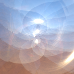 | 
[Table [importanceSamplingViz]: Importance sampling vs pre-filtered importance sampling with $\alpha = 0.4$]
The reference renderer used in the comparison below performs no approximation. In particular, it does not assume $v = n$ and does not perform the split sum approximation. The pre-filtered renderer uses all the techniques discussed in this section: pre-filtered cubemaps, the analytic formulation of the DFG term, and of course the split sum approximation.
Left: reference renderer, right: pre-filtered importance sampling.
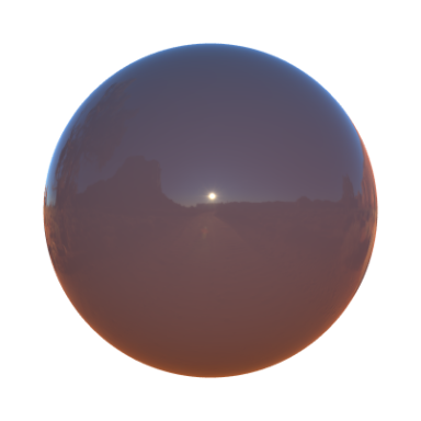 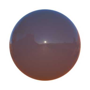
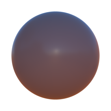 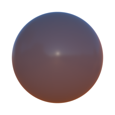
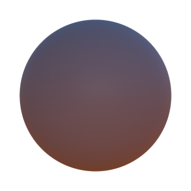 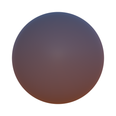
 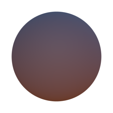
## Choosing important directions for sampling the BRDF
For simplicity we use the $ D $ term of the BRDF as the PDF, however the PDF must be normalized such that the integral over the hemisphere is 1:
$$\begin{equation}
\int_{\Omega}p(m)dm = 1 \\
\int_{\Omega}D(m)(n \cdot m)dm = 1 \\
\int_{\phi=0}^{2\pi}\int_{\theta=0}^{\frac{\pi}{2}}D(\theta,\phi) cos \theta sin \theta d\theta d\phi = 1 \\
\end{equation}$$
The PDF of the BRDF can therefore be expressed as in equation $\ref{importantPDF}$:
$$\begin{equation}\label{importantPDF}
p(\theta,\phi) = \frac{\alpha^2}{\pi(cos^2\theta (\alpha^2-1) + 1)^2} cos\theta sin\theta
\end{equation}$$
The term $sin\theta$ comes from the differential solid angle $sin\theta d\phi d\theta$ since we integrate over a sphere. We sample $\theta$ and $\phi$ independently:
$$\begin{align*}
p(\theta) &= \int_0^{2\pi} p(\theta,\phi) d\phi = \frac{2\alpha^2}{(cos^2\theta (\alpha^2-1) + 1)^2} cos\theta sin\theta \\
p(\phi) &= \frac{p(\theta,\phi)}{p(\phi)} = \frac{1}{2\pi}
\end{align*}$$
The expression of $ p(\phi) $ is true for an isotropic distribution of normals.
We then calculate the cumulative distribution function (CDF) for each variable:
$$\begin{align*}
P(s_{\phi}) &= \int_{0}^{s_{\phi}} p(\phi) d\phi = \frac{s_{\phi}}{2\pi} \\
P(s_{\theta}) &= \int_{0}^{s_{\theta}} p(\theta) d\theta = 2 \alpha^2 \left( \frac{1}{(2\alpha^4-4\alpha^2+2) cos(s_{\theta})^2 + 2\alpha^2 - 2} - \frac{1}{2\alpha^4-2\alpha^2} \right)
\end{align*}$$
We set $ P(s_{\phi}) $ and $ P(s_{\theta}) $ to random variables $ \zeta_{\phi} $ and $ \zeta_{\theta} $ and solve for $ s_{\phi} $ and $ s_{\theta} $ respectively:
$$\begin{align*}
P(s_{\phi}) &= \zeta_{\phi} \rightarrow s_{\phi} = 2\pi\zeta_{\phi} \\
P(s_{\theta}) &= \zeta_{\theta} \rightarrow s_{\theta} = cos^{-1} \sqrt{\frac{1-\zeta_{\theta}}{(\alpha^2-1)\zeta_{\theta}+1}}
\end{align*}$$
So given a uniform distribution $ (\zeta_{\phi},\zeta_{\theta}) $, our important direction $l$ is defined as:
$$\begin{align*}
\phi &= 2\pi\zeta_{\phi} \\
\theta &= cos^{-1} \sqrt{\frac{1-\zeta_{\theta}}{(\alpha^2-1)\zeta_{\theta}+1}} \\
l &= \{ cos\phi sin\theta,sin\phi sin\theta,cos\theta \}
\end{align*}$$
## Hammersley sequence
~~~~~~~~~~~~~~~~~~~~~~~~~~~~~~~~~~~~~~
vec2f hammersley(uint i, float numSamples) {
uint bits = i;
bits = (bits << 16) | (bits >> 16);
bits = ((bits & 0x55555555) << 1) | ((bits & 0xAAAAAAAA) >> 1);
bits = ((bits & 0x33333333) << 2) | ((bits & 0xCCCCCCCC) >> 2);
bits = ((bits & 0x0F0F0F0F) << 4) | ((bits & 0xF0F0F0F0) >> 4);
bits = ((bits & 0x00FF00FF) << 8) | ((bits & 0xFF00FF00) >> 8);
return vec2f(i / numSamples, bits / exp2(32));
}
~~~~~~~~~~~~~~~~~~~~~~~~~~~~~~~~~~~~~~
[C++ implementation of a Hammersley sequence generator]
## Precomputing L for image-based lighting
The term $ L_{DFG} $ is only dependent on $ \NoV $. Below, the normal is arbitrarily set to $ n=\left[0, 0, 1\right] $ and $v$ is chosen to satisfy $ \NoV $. The vector $ h_i $ is the $ D_{GGX}(\alpha) $ important direction sample $i$.
~~~~~~~~~~~~~~~~~~~~~~~~~~~~~~~~~~~~~~
float GDFG(float NoV, float NoL, float a) {
float a2 = a * a;
float GGXL = NoV * sqrt((-NoL * a2 + NoL) * NoL + a2);
float GGXV = NoL * sqrt((-NoV * a2 + NoV) * NoV + a2);
return (2 * NoL) / (GGXV + GGXL);
}
float2 DFG(float NoV, float a) {
float3 V;
V.x = sqrt(1.0f - NoV*NoV);
V.y = 0.0f;
V.z = NoV;
float2 r = 0.0f;
for (uint i = 0; i < sampleCount; i++) {
float2 Xi = hammersley(i, sampleCount);
float3 H = importanceSampleGGX(Xi, a, N);
float3 L = 2.0f * dot(V, H) * H - V;
float VoH = saturate(dot(V, H));
float NoL = saturate(L.z);
float NoH = saturate(H.z);
if (NoL > 0.0f) {
float G = GDFG(NoV, NoL, a);
float Gv = G * VoH / NoH;
float Fc = pow(1 - VoH, 5.0f);
r.x += Gv * (1 - Fc);
r.y += Gv * Fc;
}
}
return r * (1.0f / sampleCount);
}
~~~~~~~~~~~~~~~~~~~~~~~~~~~~~~~~~~~~~~
[C++ implementation of the $ L_{DFG} $ term]
## Spherical Harmonics
Symbol | Definition
:---------------------------:|:---------------------------|
$K^m_l$ | Normalization factors
$P^m_l(x)$ | Associated Legendre polynomials
$y^m_l$ | Spherical harmonics bases, or SH bases
$L^m_l$ | SH coefficients of the $L(s)$ function defined on the unit sphere
[Table [shSymbols]: Spherical harmonics symbols definitions]
### Basis functions
Spherical parameterization of points on the surface of the unit sphere:
$$\begin{equation}
\{ x, y, z \} = \{ cos \phi sin \theta, sin \phi sin \theta, cos \theta \}
\end{equation}$$
The complex spherical harmonics bases are given by:
$$\begin{equation}
Y^m_l(\theta, \phi) = K^m_l e^{im\theta} P^{|m|}_l(cos \theta), l \in N, -l <= m <= l
\end{equation}$$
However we only need the real bases:
$$\begin{align*}
y^{m > 0}_l &= \sqrt{2} K^m_l cos(m \phi) P^m_l(cos \theta) \\
y^{m < 0}_l &= \sqrt{2} K^m_l sin(|m| \phi) P^{|m|}_l(cos \theta) \\
y^0_l &= K^0_l P^0_l(cos \theta)
\end{align*}$$
The normalization factors are given by:
$$\begin{equation}
K^m_l = \sqrt{\frac{(2l + 1)(l - |m|)!}{4 \pi (l + |m|)!}}
\end{equation}$$
The associated Legendre polynomials $P^{|m|}_l$ can be calculated from the following recursions:
$$\begin{equation}\label{shRecursions}
P^0_0(x) = 1 \\
P^0_1(x) = x \\
P^l_l(x) = (-1)^l (2l - 1)!! (1 - x^2)^{\frac{l}{2}} \\
P^m_l(x) = \frac{((2l - 1) x P^m_{l - 1} - (l + m - 1) P^m_{l - 2})}{l - m} \\
\end{equation}$$
Computing $y^{|m|}_l$ requires to compute $P^{|m|}_l(z)$ first.
This can be accomplished fairly easily using the recursions in equation $\ref{shRecursions}$.
The third recursion can be used to "move diagonally" in table [basisFunctions], i.e. calculating $y^0_0$, $y^1_1$, $y^2_2$ etc.
Then, the fourth recursion can be used to move vertically.
Band index | Basis functions $-l <= m <= l$
:-----------:|:---------------------------------:|
$l = 0$ | $y^0_0$
$l = 1$ | $y^{-1}_1$ $y^0_1$ $y^1_1$
$l = 2$ | $y^{-2}_2$ $y^{-1}_2$ $y^0_2$ $y^1_2$ $y^2_2$
[Table [basisFunctions]: Basis functions per band]
It’s also fairly easy to compute the trigonometric terms recursively:
$$\begin{align*}
C_m &\equiv cos(m \phi)sin(\theta)^m \\
S_m &\equiv sin(m \phi)sin(\theta)^m \\
\{ x, y, z \} &= \{ cos \phi sin \theta, sin \phi sin \theta, cos \theta \}
\end{align*}$$
Using the angle sum trigonometric identities:
$$\begin{align*}
cos(m \phi + \phi) &= cos(m \phi) cos(\phi) - sin(m \phi) sin(\phi) \Leftrightarrow C_{m + 1} = x C_m - y S_m \\
sin(m \phi + \phi) &= sin(m \phi) cos(\phi) + cos(m \phi) sin(\phi) \Leftrightarrow S_{m + 1} = x S_m - y C_m
\end{align*}$$
Listing [nonNormalizedSHBasis] shows the C++ code to compute the non-normalized SH basis $\frac{y^m_l(s)}{\sqrt{2} K^m_l}$:
~~~~~~~~~~~~~~~~~~~~~~~~~~~~~~~~~~~~~~
static inline size_t SHindex(ssize_t m, size_t l) {
return l * (l + 1) + m;
}
void computeShBasis(
double* const SHb,
size_t numBands,
const vec3& s)
{
// handle m=0 separately, since it produces only one coefficient
double Pml_2 = 0;
double Pml_1 = 1;
SHb[0] = Pml_1;
for (ssize_t l = 1; l < numBands; l++) {
double Pml = ((2 * l - 1) * Pml_1 * s.z - (l - 1) * Pml_2) / l;
Pml_2 = Pml_1;
Pml_1 = Pml;
SHb[SHindex(0, l)] = Pml;
}
double Pmm = 1;
for (ssize_t m = 1; m < numBands ; m++) {
Pmm = (1 - 2 * m) * Pmm;
double Pml_2 = Pmm;
double Pml_1 = (2 * m + 1)*Pmm*s.z;
// l == m
SHb[SHindex(-m, m)] = Pml_2;
SHb[SHindex( m, m)] = Pml_2;
if (m + 1 < numBands) {
// l == m+1
SHb[SHindex(-m, m + 1)] = Pml_1;
SHb[SHindex( m, m + 1)] = Pml_1;
for (ssize_t l = m + 2; l < numBands; l++) {
double Pml = ((2 * l - 1) * Pml_1 * s.z - (l + m - 1) * Pml_2)
/ (l - m);
Pml_2 = Pml_1;
Pml_1 = Pml;
SHb[SHindex(-m, l)] = Pml;
SHb[SHindex( m, l)] = Pml;
}
}
}
double Cm = s.x;
double Sm = s.y;
for (ssize_t m = 1; m <= numBands ; m++) {
for (ssize_t l = m; l < numBands ; l++) {
SHb[SHindex(-m, l)] *= Sm;
SHb[SHindex( m, l)] *= Cm;
}
double Cm1 = Cm * s.x - Sm * s.y;
double Sm1 = Sm * s.x + Cm * s.y;
Cm = Cm1;
Sm = Sm1;
}
}
~~~~~~~~~~~~~~~~~~~~~~~~~~~~~~~~~~~~~~
[Listing [nonNormalizedSHBasis]: C++ implementation to compute a non-normalized SH basis]
Normalized SH basis functions $y^m_l(s)$ for the first 3 bands:
Band | $m = -2$ | $m = -1$ | $m = 0$ | $m = 1$ | $m = 2$ |
:-------:|:------------------------------------:|:-------------------------------------:|:---------------------------------------------------:|:-------------------------------------:|:---------------------------------------------:|
$l = 0$ | | | $\frac{1}{2}\sqrt{\frac{1}{\pi}}$ | | |
$l = 1$ | | $-\frac{1}{2}\sqrt{\frac{3}{\pi}}y$ | $\frac{1}{2}\sqrt{\frac{3}{\pi}}z$ | $-\frac{1}{2}\sqrt{\frac{3}{\pi}}x$ | |
$l = 2$ | $\frac{1}{2}\sqrt{\frac{15}{\pi}}xy$ | $-\frac{1}{2}\sqrt{\frac{15}{\pi}}yz$ | $\frac{1}{4}\sqrt{\frac{5}{\pi}}(2z^2 - x^2 - y^2)$ | $-\frac{1}{2}\sqrt{\frac{15}{\pi}}xz$ | $\frac{1}{4}\sqrt{\frac{15}{\pi}}(x^2 - y^2)$ |
[Table [basisFunctions]: Normalized basis functions per band]
### Decomposition and reconstruction
A function $L(s)$ defined on a sphere is projected to the SH basis as follows:
$$\begin{equation}
L^m_l = \int_\Omega L(s) y^m_l(s) ds \\
L^m_l = \int_{\theta = 0}^{\pi} \int_{\phi = 0}^{2\pi} L(\theta, \phi) y^m_l(\theta, \phi) sin \theta d\theta d\phi
\end{equation}$$
Note that each $L^m_l$ is a vector of 3 values, one for each RGB color channel.
The inverse transformation, or reconstruction, or rendering, from the SH coefficients is given by:
$$\begin{equation}
\hat{L}(s) = \sum_l \sum_{m = -l}^l L^m_l y^m_l(s)
\end{equation}$$
### Decomposition of $\left< cos \theta \right>$
Since $\left< cos \theta \right>$ does not depend on $\phi$ (azimuthal independence), the integral simplifies to:
$$\begin{align*}
C^0_l &= 2\pi \int_0^{\pi} \left< cos \theta \right> y^0_l(\theta) sin \theta d\theta \\
C^0_l &= 2\pi K^m_l \int_0^{\frac{\pi}{2}} P^0_l(cos \theta) cos \theta sin \theta d\theta \\
C^m_l &= 0, m != 0
\end{align*}$$
In [#Ramamoorthi01] an analytical solution to the integral is described:
$$\begin{align*}
C_1 &= \sqrt{\frac{\pi}{3}} \\
C_{odd} &= 0 \\
C_{l, even} &= 2\pi \sqrt{\frac{2l + 1}{4\pi}} \frac{(-1)^{\frac{l}{2} - 1}}{(l + 2)(l - 1)} \frac{l!}{2^l (\frac{l!}{2})^2}
\end{align*}$$
The first few coefficients are:
$$\begin{align*}
C_0 &= +0.88623 \\
C_1 &= +1.02333 \\
C_2 &= +0.49542 \\
C_3 &= +0.00000 \\
C_4 &= -0.11078
\end{align*}$$
Very few coefficients are needed to reasonably approximate $\left< cos \theta \right>$, as shown in figure [shCosThetaApprox].
![Figure [shCosThetaApprox]: Approximation of $cos \theta$ with SH coefficients](images/chart_sh_cos_thera_approx.png)
### Convolution
Convolutions by a kernel $h$ that has a circular symmetry can be applied directly and easily in SH space:
$$\begin{equation}
(h * f)^m_l = \sqrt{\frac{4\pi}{2l + 1}} h^0_l(s) f^m_l(s)
\end{equation}$$
Conveniently, $\sqrt{\frac{4\pi}{2l + 1}} = \frac{1}{K^0_l}$, so in practice we pre-multiply $C_l$ by $\frac{1}{K^0_l}$ and we get a simpler expression:
$$\begin{equation}
\hat{C}_{l, even} = 2\pi \frac{(-1)^{\frac{l}{2} - 1}}{(l + 2)(l - 1)} \frac{l!}{2^l (\frac{l!}{2})^2} \\
\hat{C}_1 = \frac{2\pi}{3}
\end{equation}$$
Here is the C++ code to compute $\hat{C}_l$:
~~~~~~~~~~~~~~~~~~~~~~~~~~~~~~~~~~~~~~
static double factorial(size_t n, size_t d = 1);
// < cos(theta) > SH coefficients pre-multiplied by 1 / K(0,l)
double computeTruncatedCosSh(size_t l) {
if (l == 0) {
return M_PI;
} else if (l == 1) {
return 2 * M_PI / 3;
} else if (l & 1) {
return 0;
}
const size_t l_2 = l / 2;
double A0 = ((l_2 & 1) ? 1.0 : -1.0) / ((l + 2) * (l - 1));
double A1 = factorial(l, l_2) / (factorial(l_2) * (1 << l));
return 2 * M_PI * A0 * A1;
}
// returns n! / d!
double factorial(size_t n, size_t d ) {
d = std::max(size_t(1), d);
n = std::max(size_t(1), n);
double r = 1.0;
if (n == d) {
// intentionally left blank
} else if (n > d) {
for ( ; n>d ; n--) {
r *= n;
}
} else {
for ( ; d>n ; d--) {
r *= d;
}
r = 1.0 / r;
}
return r;
}
~~~~~~~~~~~~~~~~~~~~~~~~~~~~~~~~~~~~~~
## Sample validation scene for Mitsuba
~~~~~~~~~~~~~~~~~~~~~~~~~~~~~~~~~~~~~~
<scene version="0.5.0">
<integrator type="path"/>
<shape type="serialized" id="sphere_mesh">
<string name="filename" value="plastic_sphere.serialized"/>
<integer name="shapeIndex" value="0"/>
<bsdf type="roughplastic">
<string name="distribution" value="ggx"/>
<float name="alpha" value="0.0"/>
<srgb name="diffuseReflectance" value="0.81, 0.0, 0.0"/>
</bsdf>
</shape>
<emitter type="envmap">
<string name="filename" value="../../environments/office/office.exr"/>
<float name="scale" value="35000.0" />
<boolean name="cache" value="false" />
</emitter>
<emitter type="directional">
<vector name="direction" x="-1" y="-1" z="1" />
<rgb name="irradiance" value="120000.0, 115200.0, 114000.0" />
</emitter>
<sensor type="perspective">
<float name="farClip" value="12.0"/>
<float name="focusDistance" value="4.1"/>
<float name="fov" value="45"/>
<string name="fovAxis" value="y"/>
<float name="nearClip" value="0.01"/>
<transform name="toWorld">
<lookat target="0, 0, 0" origin="0, 0, -3.1" up="0, 1, 0"/>
</transform>
<sampler type="ldsampler">
<integer name="sampleCount" value="256"/>
</sampler>
<film type="ldrfilm">
<integer name="height" value="1440"/>
<integer name="width" value="2048"/>
<float name="exposure" value="-15.23" />
<rfilter type="gaussian"/>
</film>
</sensor>
</scene>
~~~~~~~~~~~~~~~~~~~~~~~~~~~~~~~~~~~~~~
## Light assignment with froxels
Assigning lights to froxels can be implemented on the GPU using two compute shaders. The first one, shown in listing [froxelGeneration], creates the froxels data (4 planes + a min Z and max Z per froxel) in an SSBO and needs to be run only once. The shader requires the following uniforms:
Projection matrix
: The projection matrix used to render the scene (view space to clip space transformation).
Inverse projection matrix
: The inverse of the projection matrix used to render the scene (clip space to view space transformation).
Depth parameters
: $-log2(\frac{z_{lighnear}}{z_{far}}) \frac{1}{maxSlices-1}$, maximum number of depth slices, Z near and Z far.
Clip space size
: $\frac{F_x \times F_r}{w} \times 2$, with $F_x$ the number of tiles on the X axis, $F_r$ the resolution in pixels of a tile and w the width in pixels of the render target.
~~~~~~~~~~~~~~~~~~~~~~~~~~~~~~~~~~~~~~
#version 310 es
precision highp float;
precision highp int;
#define FROXEL_RESOLUTION 80u
layout(local_size_x = 1, local_size_y = 1, local_size_z = 1) in;
layout(location = 0) uniform mat4 projectionMatrix;
layout(location = 1) uniform mat4 projectionInverseMatrix;
layout(location = 2) uniform vec4 depthParams; // index scale, index bias, near, far
layout(location = 3) uniform float clipSpaceSize;
struct Froxel {
// NOTE: the planes should be stored in vec4[4] but the
// Adreno shader compiler has a bug that causes the data
// to not be read properly inside the loop
vec4 plane0;
vec4 plane1;
vec4 plane2;
vec4 plane3;
vec2 minMaxZ;
};
layout(binding = 0, std140) writeonly restrict buffer FroxelBuffer {
Froxel data[];
} froxels;
shared vec4 corners[4];
shared vec2 minMaxZ;
vec4 projectionToView(vec4 p) {
p = projectionInverseMatrix * p;
return p / p.w;
}
vec4 createPlane(vec4 b, vec4 c) {
// standard plane equation, with a at (0, 0, 0)
return vec4(normalize(cross(c.xyz, b.xyz)), 1.0);
}
void main() {
uint index = gl_WorkGroupID.x + gl_WorkGroupID.y * gl_NumWorkGroups.x +
gl_WorkGroupID.z * gl_NumWorkGroups.x * gl_NumWorkGroups.y;
if (gl_LocalInvocationIndex == 0u) {
// first tile the screen and build the frustum for the current tile
vec2 renderTargetSize = vec2(FROXEL_RESOLUTION * gl_NumWorkGroups.xy);
vec2 frustumMin = vec2(FROXEL_RESOLUTION * gl_WorkGroupID.xy);
vec2 frustumMax = vec2(FROXEL_RESOLUTION * (gl_WorkGroupID.xy + 1u));
corners[0] = vec4(
frustumMin.x / renderTargetSize.x * clipSpaceSize - 1.0,
(renderTargetSize.y - frustumMin.y) / renderTargetSize.y
* clipSpaceSize - 1.0,
1.0,
1.0
);
corners[1] = vec4(
frustumMax.x / renderTargetSize.x * clipSpaceSize - 1.0,
(renderTargetSize.y - frustumMin.y) / renderTargetSize.y
* clipSpaceSize - 1.0,
1.0,
1.0
);
corners[2] = vec4(
frustumMax.x / renderTargetSize.x * clipSpaceSize - 1.0,
(renderTargetSize.y - frustumMax.y) / renderTargetSize.y
* clipSpaceSize - 1.0,
1.0,
1.0
);
corners[3] = vec4(
frustumMin.x / renderTargetSize.x * clipSpaceSize - 1.0,
(renderTargetSize.y - frustumMax.y) / renderTargetSize.y
* clipSpaceSize - 1.0,
1.0,
1.0
);
uint froxelSlice = gl_WorkGroupID.z;
minMaxZ = vec2(0.0, 0.0);
if (froxelSlice > 0u) {
minMaxZ.x = exp2((float(froxelSlice) - depthParams.y) * depthParams.x)
* depthParams.w;
}
minMaxZ.y = exp2((float(froxelSlice + 1u) - depthParams.y) * depthParams.x)
* depthParams.w;
}
if (gl_LocalInvocationIndex == 0u) {
vec4 frustum[4];
frustum[0] = projectionToView(corners[0]);
frustum[1] = projectionToView(corners[1]);
frustum[2] = projectionToView(corners[2]);
frustum[3] = projectionToView(corners[3]);
froxels.data[index].plane0 = createPlane(frustum[0], frustum[1]);
froxels.data[index].plane1 = createPlane(frustum[1], frustum[2]);
froxels.data[index].plane2 = createPlane(frustum[2], frustum[3]);
froxels.data[index].plane3 = createPlane(frustum[3], frustum[0]);
froxels.data[index].minMaxZ = minMaxZ;
}
}
~~~~~~~~~~~~~~~~~~~~~~~~~~~~~~~~~~~~~~
[Listing [froxelGeneration]: GLSL implementation of froxels data generation (compute shader)]
The second compute shader, shown in listing [froxelEvaluation], runs every frame (if the camera and/or lights have changed) and assigns all the lights to their respective froxels. This shader relies only on a couple of uniforms (the number of point/spot lights and the view matrix) and four SSBOs:
Light index buffer
: For each froxel, the index of each light that affects said froxel. The indices for point lights are written first and if there is enough space left, the indices for spot lights are written as well. A sentinel of value 0x7fffffffu separates point and spot lights and/or marks the end of the froxel's list of lights. Each froxel has a maximum number of lights (point + spot).
Point lights buffer
: Array of structures describing the scene's point lights.
Spot lights buffer
: Array of structures describing the scene's spot lights.
Froxels buffer
: The list of froxels represented by planes, created by the previous compute shader.
~~~~~~~~~~~~~~~~~~~~~~~~~~~~~~~~~~~~~~
#version 310 es
precision highp float;
precision highp int;
#define LIGHT_BUFFER_SENTINEL 0x7fffffffu
#define MAX_FROXEL_LIGHT_COUNT 32u
#define THREADS_PER_FROXEL_X 8u
#define THREADS_PER_FROXEL_Y 8u
#define THREADS_PER_FROXEL_Z 1u
#define THREADS_PER_FROXEL (THREADS_PER_FROXEL_X * \
THREADS_PER_FROXEL_Y * THREADS_PER_FROXEL_Z)
layout(local_size_x = THREADS_PER_FROXEL_X,
local_size_y = THREADS_PER_FROXEL_Y,
local_size_z = THREADS_PER_FROXEL_Z) in;
// x = point lights, y = spot lights
layout(location = 0) uniform uvec2 totalLightCount;
layout(location = 1) uniform mat4 viewMatrix;
layout(binding = 0, packed) writeonly restrict buffer LightIndexBuffer {
uint index[];
} lightIndexBuffer;
struct PointLight {
vec4 positionFalloff; // x, y, z, falloff
vec4 colorIntensity; // r, g, b, intensity
vec4 directionIES; // dir x, dir y, dir z, IES profile index
};
layout(binding = 1, std140) readonly restrict buffer PointLightBuffer {
PointLight lights[];
} pointLights;
struct SpotLight {
vec4 positionFalloff; // x, y, z, falloff
vec4 colorIntensity; // r, g, b, intensity
vec4 directionIES; // dir x, dir y, dir z, IES profile index
vec4 angle; // angle scale, angle offset, unused, unused
};
layout(binding = 2, std140) readonly restrict buffer SpotLightBuffer {
SpotLight lights[];
} spotLights;
struct Froxel {
// NOTE: the planes should be stored in vec4[4] but the
// Adreno shader compiler has a bug that causes the data
// to not be read properly inside the loop
vec4 plane0;
vec4 plane1;
vec4 plane2;
vec4 plane3;
vec2 minMaxZ;
};
layout(binding = 3, std140) readonly restrict buffer FroxelBuffer {
Froxel data[];
} froxels;
shared uint groupLightCounter;
shared uint groupLightIndexBuffer[MAX_FROXEL_LIGHT_COUNT];
float signedDistanceFromPlane(vec4 p, vec4 plane) {
// plane.w == 0.0, simplify computation
return dot(plane.xyz, p.xyz);
}
void synchronize() {
memoryBarrierShared();
barrier();
}
void main() {
if (gl_LocalInvocationIndex == 0u) {
groupLightCounter = 0u;
}
memoryBarrierShared();
uint froxelIndex = gl_WorkGroupID.x + gl_WorkGroupID.y * gl_NumWorkGroups.x +
gl_WorkGroupID.z * gl_NumWorkGroups.x * gl_NumWorkGroups.y;
Froxel current = froxels.data[froxelIndex];
uint offset = gl_LocalInvocationID.x +
gl_LocalInvocationID.y * THREADS_PER_FROXEL_X;
for (uint i = 0u; i < totalLightCount.x &&
groupLightCounter < MAX_FROXEL_LIGHT_COUNT &&
offset + i < totalLightCount.x; i += THREADS_PER_FROXEL) {
uint currentLight = offset + i;
vec4 center = pointLights.lights[currentLight].positionFalloff;
center.xyz = (viewMatrix * vec4(center.xyz, 1.0)).xyz;
float r = inversesqrt(center.w);
if (-center.z + r > current.minMaxZ.x &&
-center.z - r <= current.minMaxZ.y) {
if (signedDistanceFromPlane(center, current.plane0) < r &&
signedDistanceFromPlane(center, current.plane1) < r &&
signedDistanceFromPlane(center, current.plane2) < r &&
signedDistanceFromPlane(center, current.plane3) < r) {
uint index = atomicAdd(groupLightCounter, 1u);
groupLightIndexBuffer[index] = currentLight;
}
}
}
synchronize();
uint pointLightCount = groupLightCounter;
offset = froxelIndex * MAX_FROXEL_LIGHT_COUNT;
for (uint i = gl_LocalInvocationIndex; i < pointLightCount;
i += THREADS_PER_FROXEL) {
lightIndexBuffer.index[offset + i] = groupLightIndexBuffer[i];
}
if (gl_LocalInvocationIndex == 0u) {
if (pointLightCount < MAX_FROXEL_LIGHT_COUNT) {
lightIndexBuffer.index[offset + pointLightCount] = LIGHT_BUFFER_SENTINEL;
}
}
}
~~~~~~~~~~~~~~~~~~~~~~~~~~~~~~~~~~~~~~
[Listing [froxelEvaluation]: GLSL implementation of assigning lights to froxels (compute shader)]
# Revisions
February 20, 2019: Cloth shading
- Removed Fresnel term from the cloth BRDF
- Removed cloth DFG approximations, replaced with a new channel in the DFG LUT
August 21, 2018: Multiscattering
- Added section [Energy loss in specular reflectance] on how to compensate for energy loss in single scattering BRDFs
August 17, 2018: Specular color
- Added section [Specular color] to explain how the base color of various metals is computed
August 15, 2018: Fresnel
- Added a description of the Fresnel effect in section [Fresnel (specular F)]
August 9, 2018: Lighting
- Added explanation about pre-exposed lights
August 7, 2018: Cloth model
- Added description of the "Charlie" NDF
August 3, 2018: First public version
# Bibliography
[#Ashdown98]: Ian Ashdown. 1998. Parsing the IESNA LM-63 photometric data file. http://lumen.iee.put.poznan.pl/kw/iesna.txt
[#Ashikhmin00]: Michael Ashikhmin, Simon Premoze and Peter Shirley. A Microfacet-based BRDF Generator. *SIGGRAPH '00 Proceedings*, 65-74.
[#Ashikhmin07]: Michael Ashikhmin and Simon Premoze. 2007. Distribution-based BRDFs.
[#Burley12]: Brent Burley. 2012. Physically Based Shading at Disney. *Physically Based Shading in Film and Game Production, ACM SIGGRAPH 2012 Courses*.
[#Estevez17]: Alejandro Conty Estevez and Christopher Kulla. 2017. Production Friendly Microfacet Sheen BRDF. *ACM SIGGRAPH 2017*.
[#Hammon17]: Earl Hammon. 217. PBR Diffuse Lighting for GGX+Smith Microsurfaces. *GDC 2017*.
[#Heitz14]: Eric Heitz. 2014. Understanding the Masking-Shadowing Function
in Microfacet-Based BRDFs. *Journal of Computer Graphics Techniques*, 3 (2).
[#Heitz16]: Eric Heitz et al. 2016. Multiple-Scattering Microfacet BSDFs with the Smith Model. *ACM SIGGRAPH 2016*.
[#Hill12]: Colin Barré-Brisebois and Stephen Hill. 2012. Blending in Detail. http://blog.selfshadow.com/publications/blending-in-detail/
[#Karis13a]: Brian Karis. 2013. Specular BRDF Reference. http://graphicrants.blogspot.com/2013/08/specular-brdf-reference.html
[#Karis13b]: Brian Karis, 2013. Real Shading in Unreal Engine 4. https://blog.selfshadow.com/publications/s2013-shading-course/karis/s2013_pbs_epic_notes_v2.pdf
[#Karis14]: Brian Karis. 2014. Physically Based Shading on Mobile. https://www.unrealengine.com/blog/physically-based-shading-on-mobile
[#Kelemen01]: Csaba Kelemen et al. 2001. A Microfacet Based Coupled Specular-Matte BRDF Model with Importance Sampling. *Eurographics Short Presentations*.
[#Krystek85]: M. Krystek. 1985. An algorithm to calculate correlated color temperature. *Color Research & Application*, 10 (1), 38–40.
[#Krivanek08]: Jaroslave Krivànek and Mark Colbert. 2008. Real-time Shading with Filtered Importance Sampling. *Eurographics Symposium on Rendering 2008*, Volume 27, Number 4.
[#Kulla17]: Christopher Kulla and Alejandro Conty. 2017. Revisiting Physically Based Shading at Imageworks. *ACM SIGGRAPH 2017*
[#Lagarde14]: Sébastien Lagarde and Charles de Rousiers. 2014. Moving Frostbite to PBR. *Physically Based Shading in Theory and Practice, ACM SIGGRAPH 2014 Courses*.
[#Lagarde18]: Sébastien Lagarde and Evgenii Golubev. 2018. The road toward unified rendering with Unity’s high definition rendering pipeline. *Advances in Real-Time Rendering in Games, ACM SIGGRAPH 2018 Courses*.
[#Lazarov13]: Dimitar Lazarov. 2013. Physically-Based Shading in Call of Duty: Black Ops. *Physically Based Shading in Theory and Practice, ACM SIGGRAPH 2013 Courses*.
[#McAuley15]: Stephen McAuley. 2015. Rendering the World of Far Cry 4. *GDC 2015*.
[#McGuire10]: Morgan McGuire. 2010. Ambient Occlusion Volumes. *High Performance Graphics*.
[#Narkowicz14]: Krzysztof Narkowicz. 2014. Analytical DFG Term for IBL. https://knarkowicz.wordpress.com/2014/12/27/analytical-dfg-term-for-ibl
[#Neubelt13]: David Neubelt and Matt Pettineo. 2013. Crafting a Next-Gen Material Pipeline for The Order: 1886. *Physically Based Shading in Theory and Practice, ACM SIGGRAPH 2013 Courses*.
[#Oren94]: Michael Oren and Shree K. Nayar. 1994. Generalization of lambert's reflectance model. *SIGGRAPH*, 239–246. ACM.
[#Pattanaik00]: Sumanta Pattanaik00 et al. 2000. Time-Dependent Visual Adaptation
For Fast Realistic Image Display. *SIGGRAPH '00 Proceedings of the 27th annual conference on Computer graphics and interactive techniques*, 47-54.
[#Ramamoorthi01]: Ravi Ramamoorthi and Pat Hanrahan. 2001. On the relationship between radiance and irradiance: determining the illumination from images of a convex Lambertian object. *Journal of the Optical Society of America*, Volume 18, Number 10, October 2001.
[#Revie12]: Donald Revie. 2012. Implementing Fur in Deferred Shading. *GPU Pro 2*, Chapter 2.
[#Russell15]: Jeff Russell. 2015. Horizon Occlusion for Normal Mapped Reflections. http://marmosetco.tumblr.com/post/81245981087
[#Schlick94]: Christophe Schlick. 1994. An Inexpensive BRDF Model for Physically-Based Rendering. *Computer Graphics Forum*, 13 (3), 233–246.
[#Walter07]: Bruce Walter et al. 2007. Microfacet Models for Refraction through Rough Surfaces. *Proceedings of the Eurographics Symposium on Rendering*.