Blindfolding DeepVariant: Surprising Insights from Hiding Information

This blog investigates the importance of various features of sequencing data to the ability to accurately call variants. Through a series of experiments where we remove single properties, or only provide a single property of sequencing data, we can get a better idea of what unique information each feature provides. We show that channels such as base quality and mapping quality bring unique information and that a channel for “supports variant” is required for multi-allelic calling. We also show that DeepVariant can learn a very indirect measure from read length distribution in order to accurately call insertions in the absence of other information.

Introduction

DeepVariant is a deep-learning-based variant caller. It uses a CNN to classify variants based on pileups of sequenced DNA fragments aligned to the candidate sites. Metadata from these reads, such as base quality or mapping quality, get encoded into separate channels, much like RGB channels of color images.

Among the latest improvements to DeepVariant is the ability to fully customize the set of channels that are passed to the model. We ran a series of ablation experiments in which we 1) removed one of the six base channels and 2) removed all but one channel. These models were effectively blind at varying degrees to information normally available to DeepVariant. We therefore expected some degradation in accuracy, but to our surprise the loss in accuracy was not uniform: we observed specific patterns of classification errors.

From these experiments we uncovered two key findings:

1. The read_supports_variant channel is critical for classifying multiallelic variants. Without it, the model cannot differentiate between homozygous alternate (1/1) and heterozygous alternate (1/2 variants.

2. In the absence of better information, DeepVariant will learn to use more subtle cues such as read length distribution to differentiate between genotypes.

Background

To classify variants, DeepVariant scans the genome for loci that may support alternate alleles. For each of these candidate sites, DeepVariant produces a pileup image of roughly 200 base pairs in which reads are stacked vertically and aligned to the reference. Sequence features are extracted and encoded into separate channels which together form the input tensor for the model. DeepVariant’s training data is composed of millions of these tensors, which are labeled with the correct genotype.

All DeepVariant models generally contain the following six base channels:

• read_base: A value is assigned to each base {A, T, G, C} within a read.
• base_quality: A position in the aligned read is colored based on the phred-scaled read quality score of the base at that position.
• mapping_quality: The entire read is colored based on the score assigned to a given read describing how well it aligns to the reference genome.
• strand: The entire read is colored based on the strand of the read (coding or template).
• read_supports_variant: The entire read is colored based on whether it supports an alternative allele or the reference.
• base_differs_from_ref: A position in the aligned read is colored based on whether it matches the aligned pair in the reference (match or mismatch).

Figure 1: A single pileup image (called an Example) composed of multiple channels.

The set of channels used by DeepVariant has changed over time. One of the earliest versions of DeepVariant encoded only four features: read_base, base_quality, strand, and base_differs_from_ref. Through trial and error, we arrived at the set of base channels listed above for all our models. In v0.5.0, we removed a channel that encoded cigar operation length (e.g. the length of a deletion or insertion event) to improve the generalizability of models. We have also added channels that are tailored towards specific sequencing platforms to improve accuracy. For example, we added a haplotype channel to our PacBio model (Release 1.1.0), and we added an insert-size channel to our Illumina models (Release 1.4.0).

Ablating Channels

In order to gain a better understanding of each channel’s contribution to overall model performance, we trained two sets of models. The first set models were each trained by ablating one of the six default channels, as illustrated below; in this example we have removed the base_differs_from_ref channel.

Figure 2(a): A pileup image with the base_differs_from_ref channel ablated.

The second set of models were trained on just a single channel chosen from the default channels. These experiments isolate the information contained in each of the channels separately. The following illustration is an example of isolating the read_base channel.

Figure 2(b): A single channel pileup image, showing only read_base information.

Included in our set of single channel experiments is a model trained on a completely blank channel (i.e. a black image). This model receives absolutely no information about any candidate and acts as a floor for expected performance.

Figure 2(c): An example of a blank channel, containing no information about reads or reference.

All models were trained using our standard GIAB Illumina WGS dataset and evaluated on HG003.

Key Findings

We first focus our attention on the ablation models, in which each model is missing one channel. These models are likely to suggest which channels encode nonredundant information.

Figure 3: F1 Scores of ablation models. Instead of the traditional six base channels, these models had one channel missing from the examples, effectively hiding the information contained in the ablated channel.

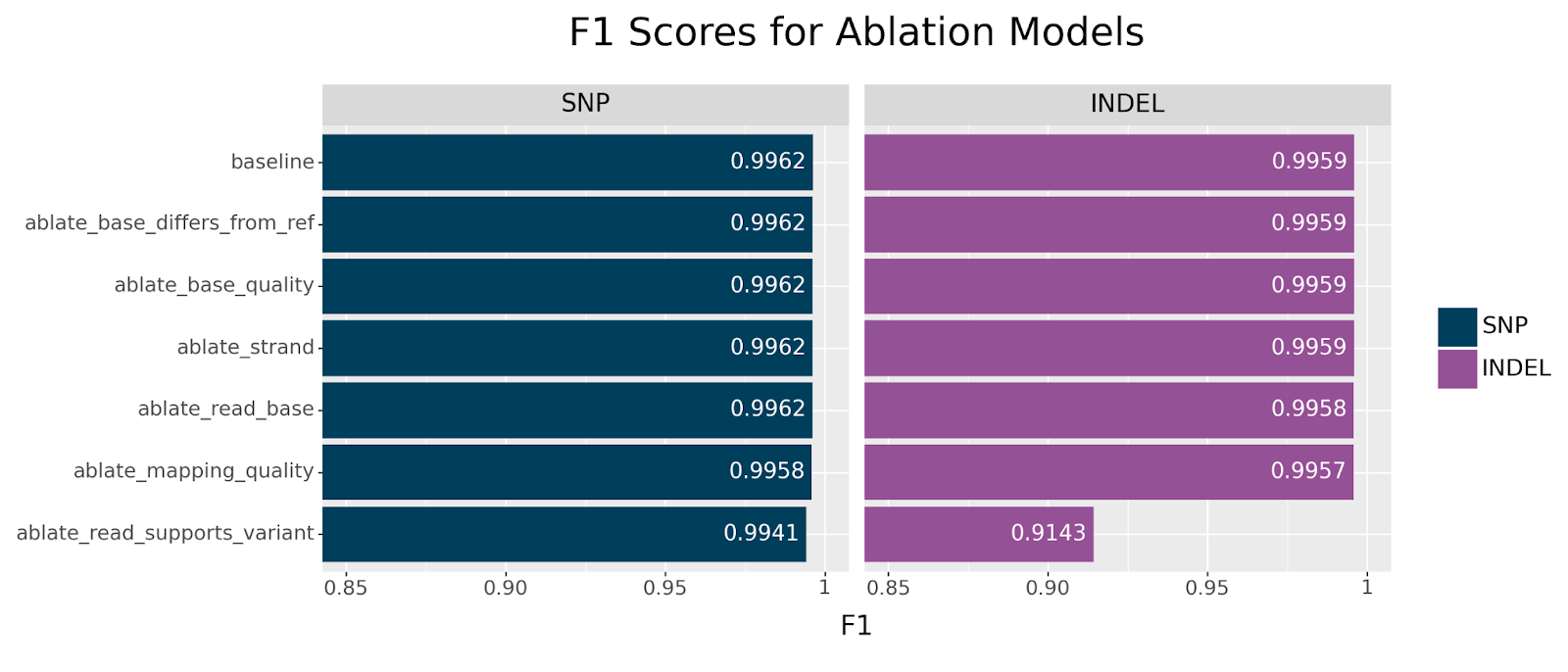
Generally speaking, we can clearly see that all models showed remarkable resilience across all ablations, especially for SNPs. The strongest decline in performance is observed for INDELs when ablating the read_supports_variant channel. This effect is also seen in SNPs but the drop is less dramatic. This suggests that this channel encodes information that is not otherwise available.

Before we try to answer what critical information the read_supports_variant channel provides, let us first consider the single channel models and see if we observe a similar effect.

Figure 4: F1 Scores of single channel models compared to baseline. Instead of the traditional six base channels, these models kept just one channel in the examples. In consequence, these models operated in a much lower information environment.

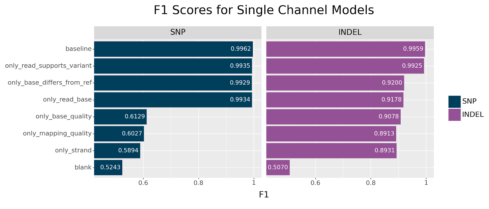
We observe the same trend in this set of experiments. The only model that performs near baseline across both SNPs and INDELs is the only_read_supports_variant model. For SNPs, we also see resilience across the base_differs_from_ref and read_base channels, but observe a precipitous drop in accuracy for the other channels. Curiously, INDELs perform reasonably well across all channels after the initial drop in accuracy.

This begs the question: what information is encoded by the read_supports_variant channel that is otherwise unavailable through other channels?

To try to answer this question, let’s break up our F1 scores by genotype. Remember that humans are diploid organisms, meaning we all have two complete sets of chromosomes, one from each parent. Broadly speaking, a variant may be classified into three genotypes:

• 0/1, i.e. heterozygous (abbreviated as het), a biallelic variant (having two observed alleles, the reference and the variant allele) where the variant allele is found on just one haplotype.
• 1/1, i.e. homozygous alternate (abbreviated as homalt), a biallelic variant where the variant allele is found on both haplotypes.
• 1/2, i.e. heterozygous alternate (abbreviated as hetalt), a multiallelic variant (having three observed alleles) where two different variant alleles are found in each haplotype.

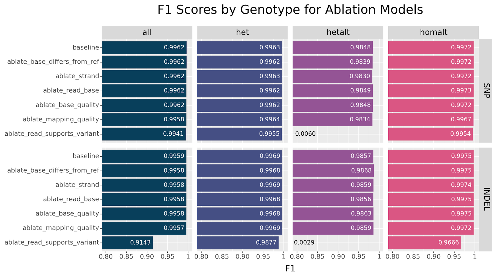
Figure 5: F1 Scores of ablation models computed per genotype, showing the global F1 score in the left most column for comparison. A clear drop in hetalt performance is observed when ablating the read_supports_variant channel.

We can see at a glance that the ablate_read_supports_variant model stands out in its failure to call hetalt variants, while all other models do not struggle with this genotype. For INDELs we also notice a slight drop in performance for the other genotypes. There is a simple explanation why the failure to correctly classify hetalt variants has different effects on SNPs versus INDELs. In our HG003 case study, hetalt variants account for 7.8% of INDELs, while they only account for 0.1% of SNPs.

Figure 6: Genotype distribution in the HG003 truth set for SNPs and INDELs.

How does DeepVariant call multiallelic loci?

The natural follow up question is why the read_supports_variant channel is critical for the model to call hetalt variants? The answer is a little tricky, and requires a deeper look at the internals of DeepVariant.

DeepVariant classifies a given example into three classes: {0/0, 0/1, 1/1}, the first describing a locus that is not a real variant (a RefCall). Consider the following example showing two SNP candidates.

Figure 7: A snapshot of an IGV alignment showing two possible SNPs, a comparatively rare multiallelic SNP being shown on the left and a more common biallelic SNP on the right.

The SNP on the right is biallelic with a reference base A and a single alternate allele C. There is one possible representation for this polymorphism: G → C, with two possible genotypes {0/1, 1/1} and therefore with three classifications (including the 0/0 case). DeepVariant produces a single pileup image for this SNP, which is sufficient to cover the three possible classifications.

In contrast, the SNP on the left is multiallelic, having two alternate alleles A and T. There are three possible polymorphisms: G → A, G → T or G → A|T, with six possible genotypes: {0/0, 0/1, 1/1, 0/2, 1/2, 2/2}. In order to get predictions for each of the six genotypes, DeepVaraint produces three examples, one for each possible representation.

To illustrate this, shown below are the three examples produced for a multiallelic insertion at chr3:163362558, purposefully stacked on top of each other.

Figure 8: The set of examples showing the three possible representations of a single multiallelic locus. Only the read_supports_variant channel encodes different information across the three examples, since it encodes if a given read supports G→A (top row), G→T (second row) or G→A|T (A or T, third row).

Notice that with the exception of read_supports_variant, all channels are exactly the same across the three examples, since they do not depend on which alternate allele is being considered. In contrast, read_supports_variant encodes if the read supports the TAC insertion, TACAC or either (in the last case). DeepVariant will classify each of those examples as some probability of ref, het or homalt, yielding 9 probabilities in total.

'chr3:163362557_T->TAC'       [0.000719, 0.999207, 0.000074]
'chr3:163362557_T->TACAC'     [0.000222, 0.999520, 0.000258]
'chr3:163362557_T->TAC|TACAC' [0.000014, 0.000112, 0.999874]

Notice how the first two examples look like and are classified as heterozygous variants, while the last one looks and is classified as a homozygous variant. With some specific logic in postprocess_variants.py, the nine probabilities are weighed together to determine that this locus presents a multiallelic variant.

Therefore, the reason why the read_supports_variant channel enables calling multiallelic variants is because it is the only channel that differentiates the possible representations of a multiallelic locus, and allows DeepVariant to resolve six genotypes in a three-class classification problem.

All other channels are identical across the different examples, and therefore unable to provide the model with the differentiating information. For example, while the read_base channel does encode the three observed alleles, DeepVariant predicts only three classes—it would need three more (0/2, 1/2, 2/2) to correctly classify them. Instead, DeepVariant relies on postprocessing to resolve these loci. However, because the predictions would be identical across the three examples—since the information is the same—this channel alone cannot differentiate between a het and a hetalt and DeepVariant chooses the former.

What if DeepVariant can “see” only a single channel?

Based on the above reasoning, we would expect to observe the same genotype-specific failures in single channel models.

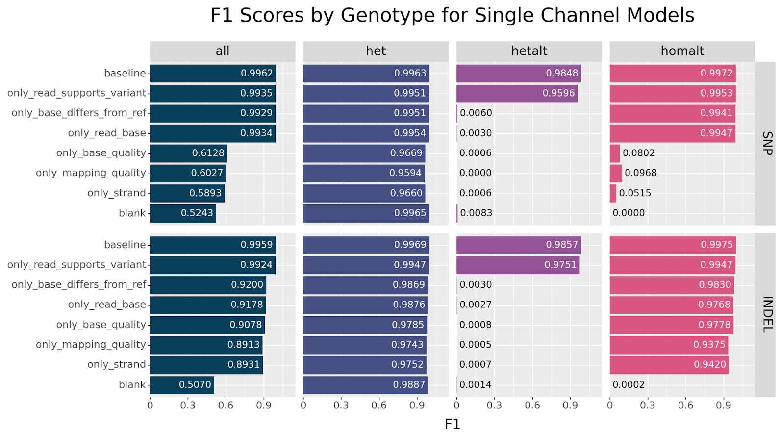
Figure 9: F1 Scores of single channel models computed per genotype, showing the global F1 score in the left most column for comparison. A clear drop in SNP homalt performance is observed for channels that do not directly encode allele information. This is not observed with INDELs.

The same pattern is observed. We can clearly see that only baseline and only_read_support_variant models are capable of classifying hetalt variants. Additionally, we observe a strong decline in homalt SNP classification when only base_quality, mapping_quality or strand information is available. Curiously, this effect is not seen with INDELs. What explains this particular drop in performance?

Before we tackle that question, we can pause briefly to address a tangential curiosity regarding the blank model: how did it achieve a F1 score of 0.52 without access to any information? We can see from Figure 11 that the answer is simple: the blank model simply calls every variant as het. This is a consequence of the fact that 1) DeepVariant is fully deterministic and will always produce the same output given the same input, and 2) heterozygous variants appear most often in our training data across both SNPs and INDELs. The model learned to minimize its loss function by always predicting this genotype.

This can be seen even more clearly when we look at the distribution of genotype predictions by each model, disregarding their correctness.

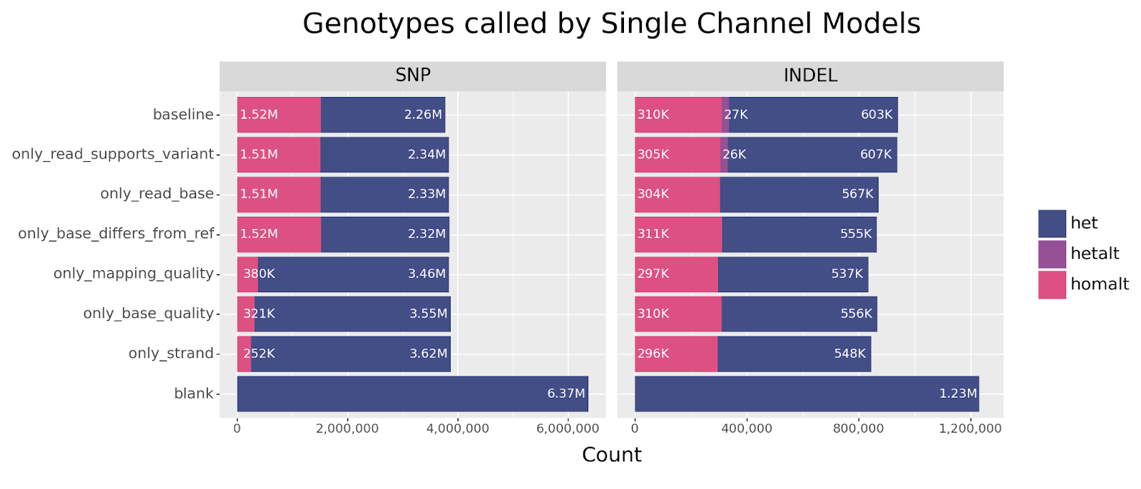
Figure 10: Absolute number of genotypes called by each model. It is clearly observed that the blank model deterministically classifies each example as het.

We also observe that for SNPs, the models with only base_quality, mapping_quality or strand information are much more likely to classify a candidate as heterozygous instead of homozygous. This begs a few questions:

1. What is it about homozygous SNPs specifically that prevent those models from calling them correctly?
2. Why is this effect not observed with INDELs?

Let’s look at the homozygous SNP chr2:522921, a G → A mutation.

Figure 11: All channel encodings of a homozygous SNP. The three channels in the top row encode allele information, while the channels in the bottom row do not.

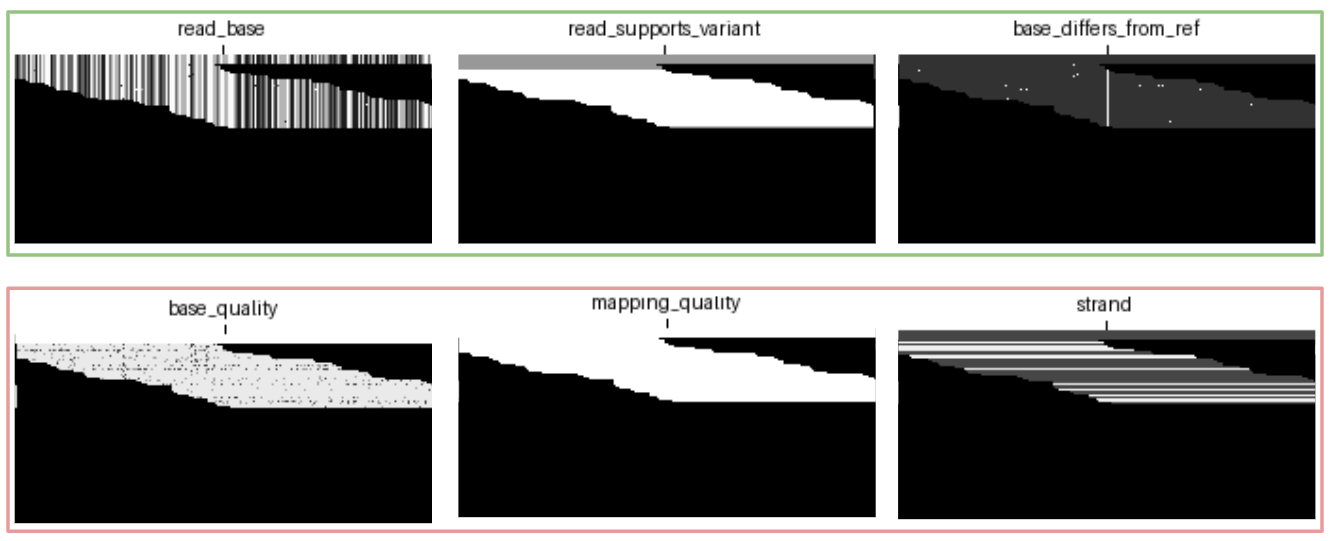
Grouped together in the top row are the three channels that encode allele information in some way:

• read_base shows a difference between the reference and alternate bases across the given reads.
• read_supports_variant shows that all reads support the given variant allele.
• base_differs_from_ref highlights all bases differ from the reference base.

Grouped together in the bottom row are channels that do not encode any allele information: base_quality, mapping_quality and strand are essentially metadata that do not convey sequence information. This answers our first question: without allele information DeepVariant cannot distinguish between a heterozygous or homozygous SNP.

So how is it possible for the bottom row models to call heterozygous variants reasonably well? Let’s look at the genotype-specific errors made by each model more closely.

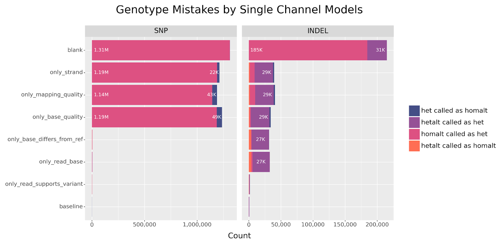
Figure 12: Absolute number of genotype mistakes made by single channel models. A clear pattern emerges that homalt SNPs are being called as het, a classification error not observed in INDELs.

The above chart looks at the composition of incorrect genotype predictions (which are counted as false negatives). We see that the models without allele information incorrectly genotype nearly all homalt SNPs as het. Similar to the blank channel, these models have learned that in the absence of differentiating signals, calling SNP candidates as het minimizes the loss function due to the abundance of this variant type. In contrast, these mistakes are minimal for models with access to allele information.

Finally, we confirm that the main source of INDEL errors come from the failure to call hetalt variants, as discussed previously. So how is it possible the same models do not struggle with INDELs in the same way?

How does DeepVariant genotype INDELs in the absence of explicit allele information?

Our last remaining puzzle to address is how all single channel models—even those that do not directly encode allele information—differentiate and classify reliably between het and homalt INDELs.

Let’s look at a pair of heterozygous and homozygous deletions that were called correctly by all models.

Figure 13: Two examples of deletions: a heterozygous deletion (top) and homozygous alternate (bottom). DeepVariant represents deletions as blank spaces within the read.

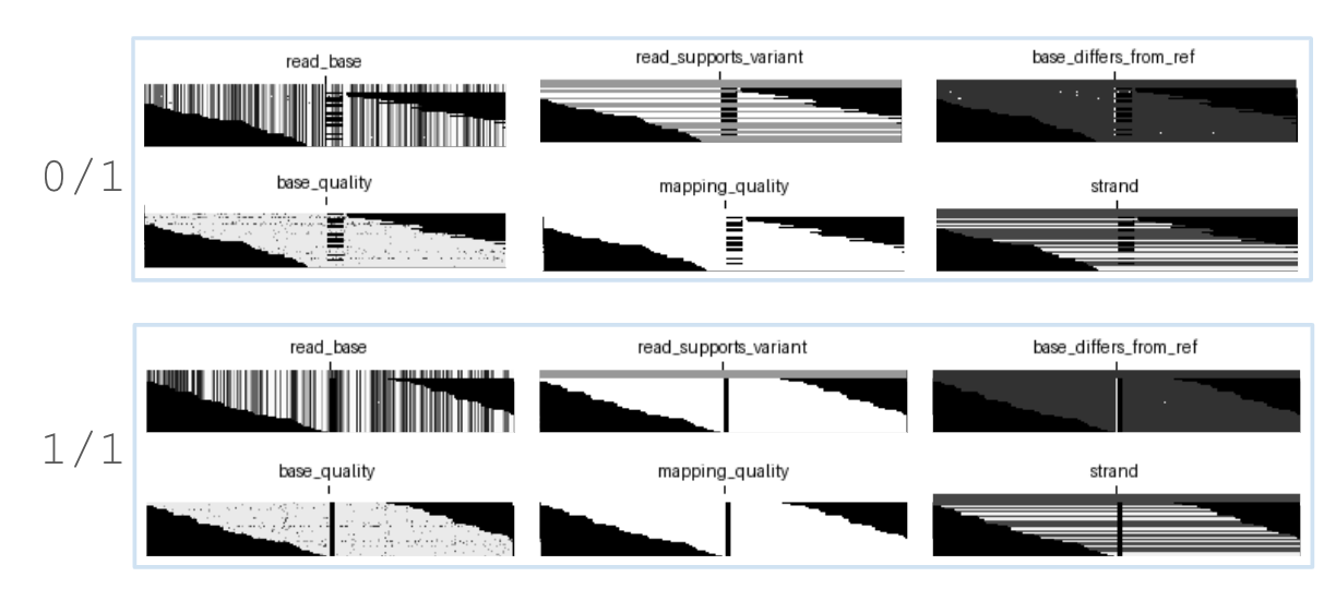
We can see that for deletions, all channels do in fact encode genotype information since deletions are represented by gaps in each read in order to maintain realignment to the reference. In this way, DeepVariant “sneaks” in extra information by how the reads are represented. Even a human could quickly classify the above deletions as 0/1 and 1/1 at a glance.

The same is not true for insertions. DeepVariant essentially encodes insertions as SNPs, showing only the first base of the insertion and dropping the rest. This again maintains alignment to the reference.

Figure 14(a): An example of an insertion illustrates how DeepVariant collapses the alternate alleles to their first base only.

Which begs the question, how is it possible for DeepVariant to call insertions reasonably well, even in the absence of allele information? Figure 16(b) illustrates how multiple insertions do not appear to contain information that would allow DeepVariant to differentiate between het and homalt if only provided with mapping_quality.

Figure 14(b): Multiple insertion loci encoded by the mapping_quality channel are shown, illustrating how they appear to contain no discernible information to differentiate genotypes (being het, homalt and het, respectively).

We would expect that the models that struggle to differentiate het and homalt SNPs would similarly struggle with insertions. To this end, let’s break up INDEL accuracy by insertion and deletion, and look at the performance across genotypes.

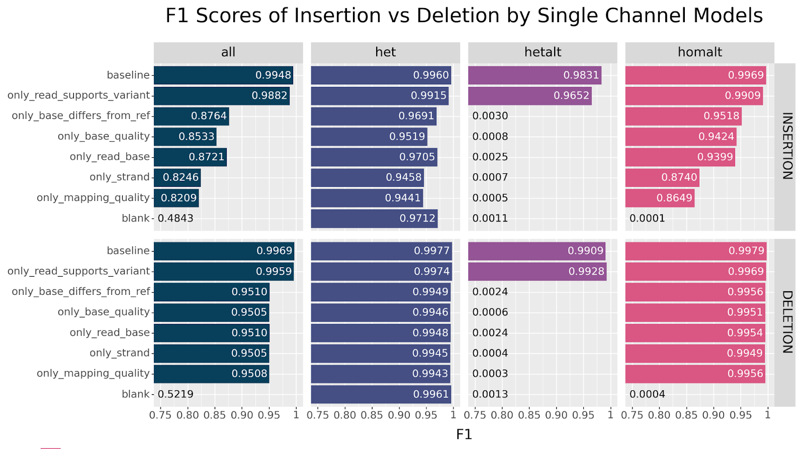
Figure 15: F1 scores of single channel models compared across insertions and deletions. There is a clear difference in homalt performance between insertion and deletions.

We can see that while the low-information models have an easier time with deletions, they still fare much better with insertions than SNPs. How is DeepVariant doing that? The examples appear to look the same between insertions and SNPs.

The answer lies in the read length distribution. Illumina short-read sequencing breaks up DNA into fragments typically 100-200 base pairs in length. For Illumina data, DeepVariant uses a 221bp width per pileup image, cropping reads if they span past the window. The represented read length distribution can be seen in Figure 17.

Figure 16: The distribution of the average read length per example across all candidates in the HG003 Illumina WGS case study.

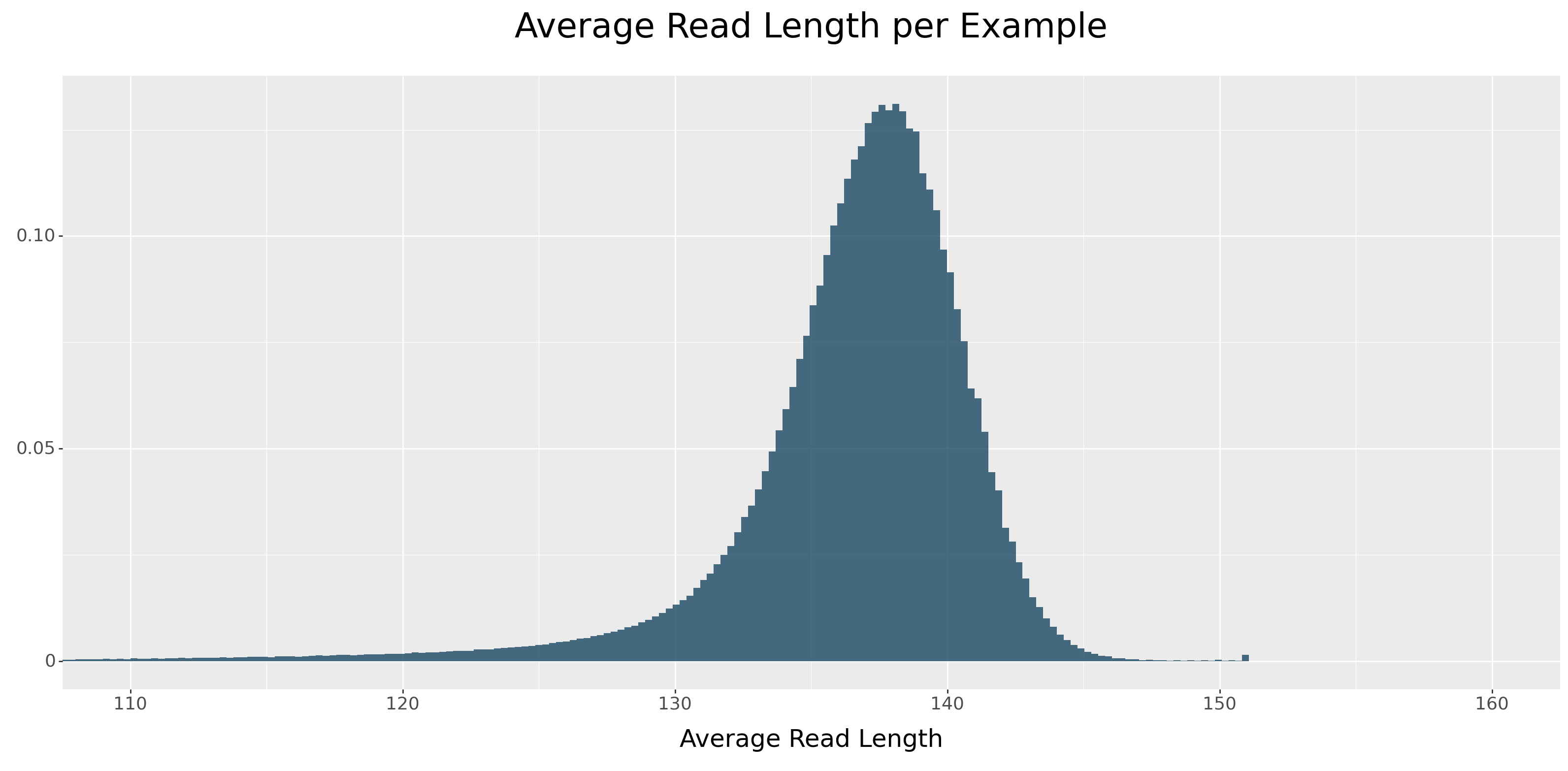
Because DeepVariant collapses the insertions—that is, representing them by their first base only—it effectively shortens them. The consequence is that reads containing insertions tend to be shorter in the pileup image. If we group the above distribution by variant type, we see a clear separation by read length across insertion size.

Figure 17: The distribution of the average read length per example broken down by SNP, deletion, and multiple ranges of insertion sizes (1-5, 6-10, 11-15, and 15+, respectively).

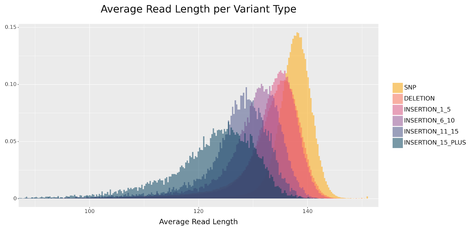
Furthermore, since het and homalt differ in the number of reads supporting the variant, a homozygous insertion will have a stronger distribution shift than a heterozygous insertion. This effect is clearly observed when comparing the read length distribution between the two genotypes.

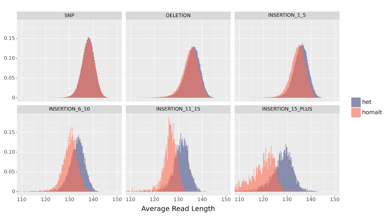
Figure 18: The distribution of the average read length per example comparing het vs homalt variants, across SNP, deletion, and multiple ranges of insertion sizes.

It follows that DeepVariant uses this information to correctly differentiate between het and homalt insertions.

Finally, we can compare the read length distribution in examples that DeepVariant classified correctly (TP) with those producing errors (FN or FP). If the model learned to use the read length distribution in the example as an indicator for genotype, we would expect that canonical examples—those that follow the above distribution shift—to be called correctly. We would expect that examples that get misclassified to deviate from this distribution.

For example, suppose the only_mapping_quality model encounters an example with a shortened read length distribution. The model would assign a higher probability to this being a homalt insertion than a het. However, it happens to be an example for a het variant composed of reads that randomly happen to be shorter than average—the result is a FN, a misclassification. Therefore, we may expect that FN+FP generally have the opposite distribution than TPs.

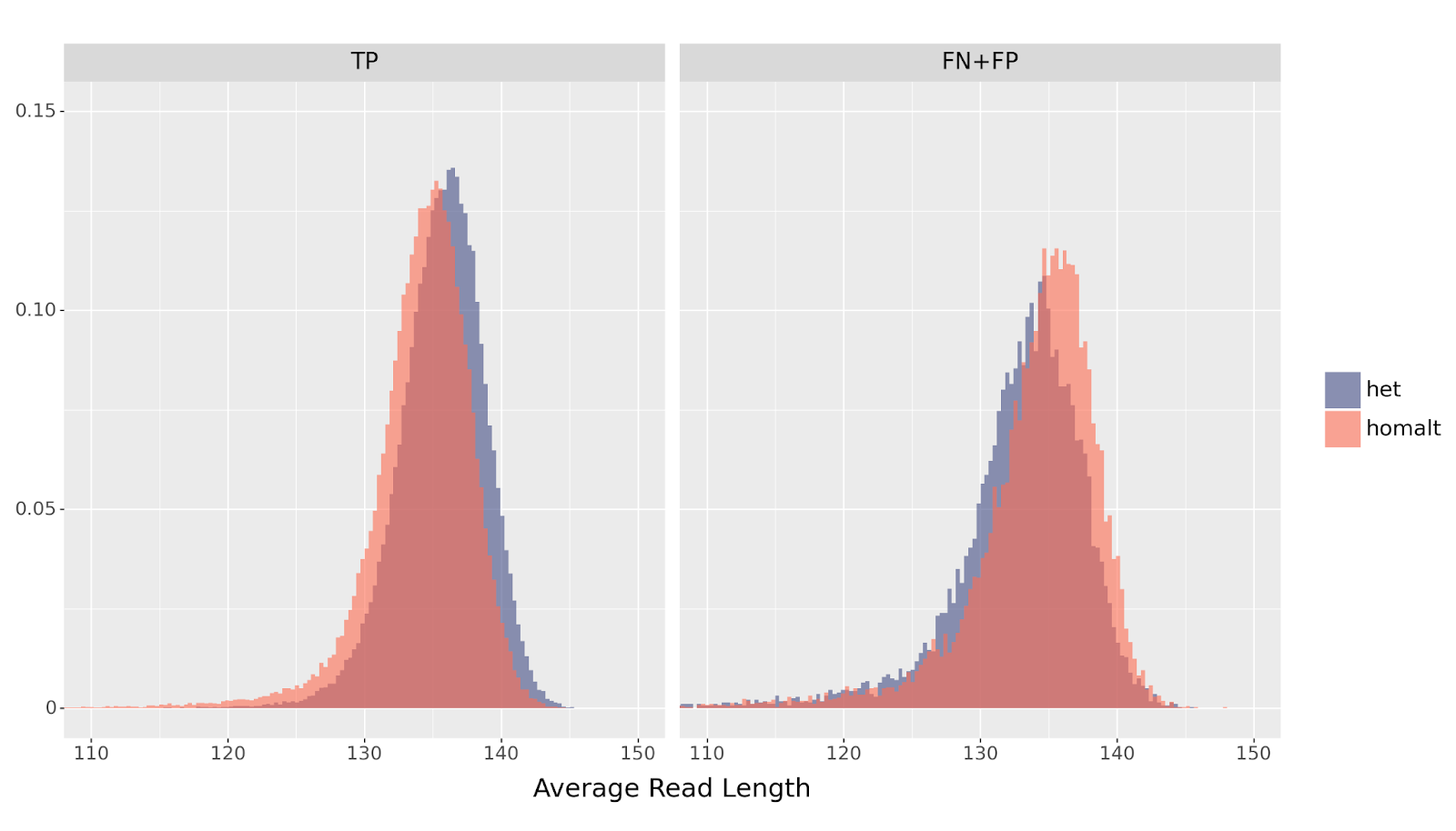
Figure 19: The distribution of the average read length per example comparing het vs homalt variants across errors (FP+FN) and TPs. A higher mean for homalt errors suggests that DeepVariant incorrectly classifies them according to the read length distribution.

The results of this analysis suggest that DeepVariant’s CNN is adept at picking up as many visual signals as possible. In the absence of rich visual information, DeepVariant will use indirect clues to minimize its loss function during training. While the read_supports_variant channel is critical for multiallelic variants, representational information such as read length distribution also allows DeepVariant to differentiate the genotypes of insertions.

Acknowledgements

We thank Maria Nattestad for a great deal of initial work developing concepts and initial explorations with channel ablation and modification. Maria’s early investigations also led to improvements such as the ALT-aligned channel by noticing the importance of the reads_supports_variant channel and identifying ways to expand the information provided there.