Signal to Noise Ratio
The Signal to Noise Ratio (SNR) (see Signal-to-noise ratio (Wikipedia)) is a classical method how to find out which time points in the trace are interesting. And how much is the signal dampened by the noise.
A Little Theory
Section titled “A Little Theory”We attempt to give the minimal necessary background. Unfortunately the ChipWhisperer tutorial on SNR keeps moving around. PA_Intro_3-Measuring_SNR_of_Target.ipynb. The use of SNR appeared in the paper
Mangard, S. (2004).Hardware countermeasures against DPA–a statistical analysis of their effectiveness.In Topics in Cryptology–CT-RSA 2004: The Cryptographers’ Track at the RSAConference 2004, San Francisco, CA, USA, February 23-27, 2004, Proceedings (pp.222-235). Springer Berlin Heidelberg.And then many more times.
For a full introduction to side channel attacks one can visit their local library or buy the amazing book The Hardware Hacking Handbook: Breaking Embedded Security with Hardware Attacks by Jasper van Woudenberg and Colin O’Flynn.
Minimum SNR Knowledge
Section titled “Minimum SNR Knowledge”One can suspect that power consumption or electromagnetic emissions at some point in time is a function of some value or its Hamming weight (Wikipedia). If this value is also connected to a secret we want to know we may try to use this correlation to uncover the secret value.
One such value which works particularly well namely for software implementation is a byte of the S-BOX input (or output). During the first round its value is the plaintext byte xored with the secret key. We know the plaintext and want to deduce the key (thus this value is connected with the secret).
Suppose that we have a profiling dataset (train or test — we know both plaintext and key) and we want to know which exact time points in the trace are changing when the value of S-BOX input is changing.
Physical measurements are never 100% clean. Thus even when at some point of time the power consumption would be a function of the byte value (or it’s Hamming weight) we would measure that affected by some noise. Often practitioners assume that the noise is independent of other bytes and normally distributed.
In many signal processing applications Signal-to-noise ratio (Wikipedia) is used. The definition (in dB — decibel) is as follows:
The power of two is there because usually in signal processing we are interested in the energy of a signal (noise) rather than it’s square root.
Let us decode the intuition of Signal and Noise. Within one class of traces (let us say all of the traces where Hamming weight of the first byte of S-BOX input is equal to 3) our assumption is that some point (or multiple points) of the trace is a deterministic function of the value 3 plus some random noise. Variance (or sample variance) is thus easy to compute — just the variance of each time point over all traces with Hamming weight of the first S-BOX input byte equal to 3. Thus we have 9 arrays (Hamming weight of a byte is 0 to 8) of variances, each of the same length as the original trace.
We often assume the additive noise caused by the measurements has mean zero and is independent from trace to trace (exercise: explain why both are reasonable assumptions). We can define variance of the signal as the variance between each class. Since we captured many traces for each class we just compute 9 sample means and compute variance of these 9 means (again an array of length equal to the length of original trace).
For our actual computation we pick the noise of the most common class (where we have the most examples to compute the variance). This is done so that the variance caused by the signal does not contribute to the noise variance.
We thus see that we need to keep track of mean and variances (for a limited number of classes). These can be done using a single pass over the data with Welford’s online algorithm (Wikipedia).
A First Try
Section titled “A First Try”The SCAAML package implements a version of the online algorithm. It uses pure NumPy and is rather conservative with regards to numerical errors (e.g., using Kahan-Babuska sum algorithm for summing).
When we run the vanilla NumPy algorithm on the "test" split of TinyAES dataset
import numpy as npfrom tqdm import tqdm
from scaaml.stats.snr import SNRSinglePassfrom scaaml.stats.attack_points.aes_128.attack_points import ( LeakageModelAES128, SubBytesIn, SubBytesOut,)from sedpack.io import Dataset
# Load the datasetdataset = Dataset(dataset_path)
snr = SNRSinglePass( leakage_model=LeakageModelAES128( byte_index=0, attack_point=SubBytesIn(), use_hamming_weight=True, ), db=True,)
split = "test"
for example in tqdm( dataset.as_numpy_iterator( split=split, repeat=False, shuffle=0, ), desc=f"[NP] Computing SNR over {split}", total=dataset._dataset_info.splits[split].number_of_examples,): snr.update(example)
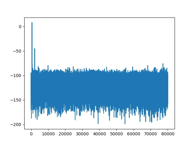
plt.plot(snr.result)plt.savefig("tiny_aes_snr_sbi_0.png")we get the following SNR (in decibels):
Time Measurements
Section titled “Time Measurements”This is not a proper benchmark. The tradeoffs for different trace lengths might differ.
On our computer (AMD Ryzen™ 9 CPU and SSD) it took around two minutes to compute SNR. We may wonder if this is caused by the data storage being slow or by our naive SNR implementation. Let us just iterate through the data and find out.
# Same iteration as before without computation.for example in tqdm( dataset.as_numpy_iterator( split=split, repeat=False, shuffle=0, ), desc=f"[NP] Computing SNR over {split}", total=dataset._dataset_info.splits[split].number_of_examples,): passJust iterating took 8 seconds (around 15 times faster with 3700 iterations per second vs previous 250). And spoiler alert we are working on improving our implementation to allow even faster iteration.
Pareto principle (Wikipedia) tells us that we should speed up the computation.
Possible Improvement Strategies
Section titled “Possible Improvement Strategies”We have seen that we are bounded by compute. There are many ways how to improve this and by no chance can we cover them all here or provide a comprehensive benchmark. Our point is quite opposite: sedpack should allow fast iteration of data in an interoperable way. That way others can focus on finding new ways to improve and optimize the data processing and build great tools. At the same time the improvements we provide here might not be the most optimal versions.
There are two main ineffective pieces of code in our previous example.
- Recomputing AES in software. The
SNRSinglePassclass withLeakageModelAES128are generic but are not optimized at all. Most notably they implement AES128 in Python even when we care about a single byte. Luckily we have savedsub_bytes_intogether with our dataset so that we may use that directly. - The
SNRSinglePassusesfloat64and numerically stable algorithms. We can get around with using pure sum.
The following code is there to show how separating the iteration and the statistical algorithm allows to easily profile. Also notice how similar the solutions are (just depending on what is currently available — GPU or not).
We just implement the Welford’s algorithm update in NumPy.
Numba is a popular way to accelerate Python code using just in time compiler (JIT).
In case we have a supported GPU accelerator we can leverage its capabilities. JAX is a popular choice for high performance array computing. One of the main advantages is that JAX API mostly follows NumPy API with a few exceptions most notably JAX embraces immutability and more functional style of programming.
One could also think about JAX automatic vectorization if they are careful which values they update (all examples in the batch need to belong to the same value class — in our example Hamming weight of the first byte of S-BOX input). We omit this direction in this tutorial.
The code for updates in Welford’s algorithms looks like follows:
# https://en.wikipedia.org/wiki/Algorithms_for_calculating_variance# Welford's algorithm
def np_update(existing_aggregate, new_trace):    """For a given value `new_trace`, compute the new `count`, new `mean`, and    new `squared_deltas`. The variables have the following meaning:
    - `mean` accumulates the mean of the entire dataset,    - `squared_deltas` aggregates the squared distance from the mean,    - `count` aggregates the number of samples seen so far.    """    (count, mean, squared_deltas) = existing_aggregate    count += 1    delta = new_trace - mean    mean += delta / count    updated_delta = new_trace - mean    squared_deltas += delta * updated_delta    return (count, mean, squared_deltas)
def np_get_initial_aggregate(trace_len: int):    dtype = np.float32    count = np.array(0, dtype=dtype)    mean = np.zeros(trace_len, dtype=dtype)    squared_deltas = np.zeros(trace_len, dtype=dtype)    return (count, mean, squared_deltas)
def np_finalize(existing_aggregate):    """Retrieve the mean and variance from an aggregate.    """    (count, mean, squared_deltas) = existing_aggregate    assert count >= 2    (mean, variance) = (mean, squared_deltas / count)    return (mean, variance)
# https://en.wikipedia.org/wiki/Algorithms_for_calculating_variance# Welford's algorithm
@numba.jitdef numba_update(existing_aggregate, new_trace): """For a given value `new_trace`, compute the new `count`, new `mean`, and new `squared_deltas`. The variables have the following meaning:
- `mean` accumulates the mean of the entire dataset, - `squared_deltas` aggregates the squared distance from the mean, - `count` aggregates the number of samples seen so far. """ (count, mean, squared_deltas) = existing_aggregate count += 1 delta = new_trace - mean mean += delta / count updated_delta = new_trace - mean squared_deltas += delta * updated_delta return (count, mean, squared_deltas)
def numba_get_initial_aggregate(trace_len: int): dtype = np.float32 count = np.array(0, dtype=dtype) mean = np.zeros(trace_len, dtype=dtype) squared_deltas = np.zeros(trace_len, dtype=dtype) return (count, mean, squared_deltas)
def numba_finalize(existing_aggregate): """Retrieve the mean and variance from an aggregate. """ (count, mean, squared_deltas) = existing_aggregate assert count >= 2 (mean, variance) = (mean, squared_deltas / count) return (mean, variance)# https://en.wikipedia.org/wiki/Algorithms_for_calculating_variance# Welford's algorithm
@jax.jitdef jax_update(existing_aggregate, new_trace): """For a given value `new_trace`, compute the new `count`, new `mean`, and new `squared_deltas`. The variables have the following meaning:
- `mean` accumulates the mean of the entire dataset, - `squared_deltas` aggregates the squared distance from the mean, - `count` aggregates the number of samples seen so far. """ (count, mean, squared_deltas) = existing_aggregate count += 1 delta = new_trace - mean mean += delta / count updated_delta = new_trace - mean squared_deltas += delta * updated_delta return (count, mean, squared_deltas)
def jax_get_initial_aggregate(trace_len: int): dtype = jnp.float32 count = jnp.array(0, dtype=dtype) mean = jnp.zeros(trace_len, dtype=dtype) squared_deltas = jnp.zeros(trace_len, dtype=dtype) return (count, mean, squared_deltas)
def jax_finalize(existing_aggregate): """Retrieve the mean and variance from an aggregate. """ (count, mean, squared_deltas) = existing_aggregate assert count >= 2 (mean, variance) = (mean, squared_deltas / count) return (mean, variance)To wrap this up in a full SNR computation:
def snr_np_welford(dataset_path: Path, ap_name: str) -> npt.NDArray[np.float32]:    """Compute SNR using NumPy.    """    # Load the dataset    dataset = Dataset(dataset_path)
    # We know that trace1 is the first.    trace_len: int = dataset.dataset_structure.saved_data_description[0].shape[0]
    leakage_to_aggregate = {        i: np_get_initial_aggregate(trace_len=trace_len) for i in range(9)    }
    split = "test"
    for example in tqdm(            dataset.as_numpy_iterator(                split=split,                repeat=False,                shuffle=0,            ),            desc=f"[NP Welford] Computing SNR over {split}",            total=dataset._dataset_info.splits[split].number_of_examples,    ):        current_leakage = int(example[ap_name][0]).bit_count()        leakage_to_aggregate[current_leakage] = np_update(leakage_to_aggregate[current_leakage], example["trace1"],)
    results = {        leakage: np_finalize(aggregate) for leakage, aggregate in leakage_to_aggregate.items()    }
    # Find out which class is the most common.    most_common_leakage = 0    most_common_count = 0    for leakage, (count, _mean, _squared_deltas) in leakage_to_aggregate.items():        if count >= most_common_count:            most_common_leakage = leakage            most_common_count = count
    signals = np.array([mean for mean, _variance in results.values()])
    return 20 * np.log(np.var(signals, axis=0) / results[most_common_leakage][1])
def snr_numba(dataset_path: Path, ap_name: str) -> npt.NDArray[np.float32]: """Compute SNR using NumPy. """ # Load the dataset dataset = Dataset(dataset_path)
# We know that trace1 is the first. trace_len: int = dataset.dataset_structure.saved_data_description[0].shape[0]
leakage_to_aggregate = { i: numba_get_initial_aggregate(trace_len=trace_len) for i in range(9) }
split = "test"
for example in tqdm( dataset.as_numpy_iterator( split=split, repeat=False, shuffle=0, ), desc=f"[Numba] Computing SNR over {split}", total=dataset._dataset_info.splits[split].number_of_examples, ): current_leakage = int(example[ap_name][0]).bit_count() leakage_to_aggregate[current_leakage] = numba_update(leakage_to_aggregate[current_leakage], np.array(example["trace1"], dtype=np.float32),)
results = { leakage: numba_finalize(aggregate) for leakage, aggregate in leakage_to_aggregate.items() }
# Find out which class is the most common. most_common_leakage = 0 most_common_count = 0 for leakage, (count, _mean, _squared_deltas) in leakage_to_aggregate.items(): if count >= most_common_count: most_common_leakage = leakage most_common_count = count
signals = np.array([mean for mean, _variance in results.values()])
return 20 * np.log(np.var(signals, axis=0) / results[most_common_leakage][1])def snr_jax(dataset_path: Path, ap_name: str) -> None: """Compute SNR using NumPy. """ # Load the dataset dataset = Dataset(dataset_path)
# We know that trace1 is the first. trace_len: int = dataset.dataset_structure.saved_data_description[0].shape[0]
leakage_to_aggregate = { i: jax_get_initial_aggregate(trace_len=trace_len) for i in range(9) }
split = "test"
for example in tqdm( dataset.as_numpy_iterator( split=split, repeat=False, shuffle=0, ), desc=f"[JAX] Computing SNR over {split}", total=dataset._dataset_info.splits[split].number_of_examples, ): current_leakage = int(example[ap_name][0]).bit_count() leakage_to_aggregate[current_leakage] = jax_update(leakage_to_aggregate[current_leakage], example["trace1"],)
results = { leakage: jax_finalize(aggregate) for leakage, aggregate in leakage_to_aggregate.items() }
# Find out which class is the most common. most_common_leakage = 0 most_common_count = 0 for leakage, (count, _mean, _squared_deltas) in leakage_to_aggregate.items(): if count >= most_common_count: most_common_leakage = leakage most_common_count = count
signals = np.array([mean for mean, _variance in results.values()])
return 20 * np.log(np.var(signals, axis=0) / results[most_common_leakage][1])Gives us the following speedups:
| Original | NP Welford | Numba | JAX |
|---|---|---|---|
| 135s | 24s | 23s | 15s |
With the maximal absolute difference being 0.058 due to numerical errors.
As we have already noted we are working on improving our Rust library for reading. At the time of writing this tutorial the read speed is roughly doubled. We expect the speedup to further improve.
Different Programming Languages
Section titled “Different Programming Languages”One might use choose another programming language than Python. We do not explore this path further. We just note that there is an excellent support for C++ in FlatBuffers. Moreover the format is simple enough to parse in other languages (e.g., Fortran). The other choice TFRecord is based on Protocol Buffers and thus also parseable in many languages. Last but not least metadata is stored in JSON files which again is highly portable.
We are using the Rust programming language to implement reading and parsing of shard files. Thus reading the raw data is easy. On the other hand the API is rather low-level and we currently do not plan a standalone Rust version of sedpack.
For instance for the Julia programming language there are both npz and flatbuffer parsers. One might in theory create a whole version of sedpack implemented in Julia. Currently we are not planning to implement this ourselves.
Other Tools
Section titled “Other Tools”The numbers here are by no means a complete benchmark. Other tools also have many more capabilities than just SNR. Last but not least the tradeoffs for different trace lengths are impossible to predict and have to be measured.