Bayesian Instrumental Variable analysis for Continuous Outcomes
Yichi Zhang
Gaussian.RmdMotivation
What is the challenge?
Randomized experiments are the gold standard for impact measurement. However, it is common that the treatment of interest can not be enforced, like the usage of a feature, or participation in a program. Instead, nudges, invites, recommendations, or encouragements are randomly assigned to induce the treatment of interest. This type of experiment design unlocks opportunities to measure the impact of numerous unenforceable treatments, but introduces a noncompliance problem: whether units adopt the treatment assigned to them is not guaranteed and subject to unobserved confounding bias.
Suppose the assignment is \(Z\) (\(Z = 1\) if nudged, \(0\) otherwise), the potential treatment adoption is \(D(Z=z) = D(z)\) (\(D = 1\) if adopted, \(0\) otherwise), and the potential outcome is \(Y(Z=z) = Y(z)\). There are four principal strata in this setting:
- Compliers: \(D(1) = 1\), \(D(0) = 0\), units who adopt the treatment when nudged, and do not adopt otherwise.
- Never-takers: \(D(1) = D(0) = 0\), units who never adopt the treatment regardless of nudges.
- Always-takers: \(D(1) = D(0) = 1\), units who always adopt the treatment regardless of nudges.
- Defiers: \(D(1) = 0\), \(D(0) = 1\), units who do the opposite of what they are nudged to do.
Compliers and defiers are the subgroups for which the impact of the treatment is well-defined and provide us with information measuring it. It is up to the study design and the collected data that some of the subpopulations may be assumed to nonexist. For example, it is common to assume no defiers. In this case, only compliers will be the target population for impact measurement.
What does not work?
This noncompliance setting with unobserved confounders deems some traditional approaches biased or irrelevant.
- The Intention to Treat (ITT) analysis contrasts the average outcomes by treatment assignment, ignoring the actual treatment adoption. It estimates the impact of the nudge, not the treatment feature.
\[ \hat{ITT} = \hat{E}[Y_i(1) - Y_i(0)] = \hat{E}[Y_i|Z_i=1] - \hat{E}[Y_i|Z_i=0] = \frac{\sum_{i=1}^n Y_i Z_i}{\sum_{i=1}^n Z_i} - \frac{\sum_{i=1}^n Y_i (1-Z_i)}{\sum_{i=1}^n (1-Z_i)}. \]
- The per-protocol analysis contrasts the average outcomes by treatment assignment, discarding noncompliant units, so treatment assignment is the same as treatment adopted. It compares two different populations. The treatment group is the mixture of compliers and always-takers, and the control group is the mixture of compliers and never-takers. It can hardly be interpreted as any causal impact since the target population is unclear.
\[ \hat{PP} = \hat{E}[Y_i|Z_i=1, D_i = 1] - \hat{E}[Y_i|Z_i=0, D_i = 0] = \frac{\sum_{i=1}^n Y_i Z_i D_i}{\sum_{i=1}^n Z_i D_i} - \frac{\sum_{i=1}^n Y_i (1-Z_i) (1-D_i)}{\sum_{i=1}^n (1-Z_i) (1-D_i)}. \]
- The as-treated analysis contrasts the average outcomes by treatment adopted, ignoring the treatment assignment. It also compares two different mixtures of subpopulations. An OLS extension further includes other observed covariates \(X\). It is still biased because the treatment adopted is not random and confounded by unobserved confounders.
\[ \hat{AT}_1 = \hat{E}[Y_i|D_i = 1] - \hat{E}[Y_i|D_i = 0] = \frac{\sum_{i=1}^n Y_i D_i}{\sum_{i=1}^n D_i} - \frac{\sum_{i=1}^n Y_i (1-D_i)}{\sum_{i=1}^n (1-D_i)}, \]
or
\[ Y_i = \beta_0 + \beta_1 D_i + \beta_2 X_i + \epsilon_i, \hat{AT}_2 = \hat{\beta}_1. \]
What works?
To address this prominent obstacle towards impact measurement, this example employs Bayesian instrumental variable analysis (BIVA) for continuous outcomes. The intuition of an IV approach is to find an exogenous variable that affects the treatment, and the outcome only through the treatment, so that the effect of the treatment on the outcome, confounded by other unobserved variables, can be disentangled through the “IV-treatment-outcome” pathway.
Aside from no defiers, the following assumptions are made about the nudge to justify its qualification as an IV:
- Random assignment: The assigned nudge is random.
- Nonzero effect on the treatment: The assigned nudge has a nonzero impact on the treatment adopted.
- Exclusion restriction (ER): The assigned nudge does not directly affect the outcome if not through the treatment adopted.
The first assumption holds by design. The second assumption could be tested. The third assumption is untestable but it is possible to relax the assumption as a sensitivity analysis in a Bayesian approach.
The implications of these assumptions are:
- The effect of the nudge on the adopted treatment and the outcome can be measured.
- The proportion of compliers is nonzero.
- The effect of the nudge on the outcome is zero among always-takers and never-takers. The effect of the nudge on the outcome is interpreted as the impact of the treatment feature among compliers.
There are two types of methods that execute the IV analysis. They both attempt to recover a local effect of the treatment among compliers called the complier average causal effect (CACE) but with different granularity. The first type of method is a global approach that does not seek to model the individual membership to the principal strata or the outcome by strata. They estimate the proportion of compliers, which dilutes the CACE of the treatment to be the ITT effect of the nudge. In other words, the proportion of compliers is the variation in the treatment adoption explained by the nudge, that multiplies the effect of the treatment on the outcome among compliers to be the variation in the outcome explained by the nudge. Representative methods in this category include the two-stage least squares (2SLS) and the frequentist moments estimate by principal stratification. They intend to recover the following quantity:
\[ \hat{CACE_1} = \hat{E}_1[Y_i(1) - Y_i(0)|D_i(1) = 1, D_i(0) = 0] = \frac{\hat{E}[Y_i|Z_i=1] - \hat{E}[Y_i|Z_i=0]} {\hat{E}[D_i|Z_i=1] - \hat{E}[D_i|Z_i=0]}. \]
The second type of method imposes models to the principal strata and outcomes by each strata-nudge combination. Within each strata, the uptake pattern of the treatment is deterministic and homogenous, so the confounded relationship between the treatment adoption and the outcome is fixed and disentangled. The nudge will fully explain the variation in the treatment adoption within each strata. The marginal variation of the treatment adoption explained by the nudge, i.e, the proportion of compliers, stems from each unit’s probability of being a complier by the strata membership model. The model parameters are jointly estimated by a frequentist maximum likelihood approach or a Bayesian approach. The likelihood looks like the following:
\[ \prod_{i: Z_i = 0, D_i = 0} (\pi_{i,c} f_{i,c0} + \pi_{i,n} f_{i,n0}) \prod_{i: Z_i = 1, D_i = 1} (\pi_{i,c} f_{i,c1} + \pi_{i,a} f_{i,a1}) \prod_{i: Z_i = 0, D_i = 1} \pi_{i,a} f_{i,a0} \prod_{i: Z_i = 1, D_i = 0} \pi_{i,n} f_{i,n1}, \]
where \(c\) stands for compliers, \(a\) for always-takers, \(n\) for never-takers, \(\pi_{i,g}\) is the probability of unit \(i\) being in strata \(g\), and \(f_{i,gz}\) is the outcome model for unit \(i\) in strata \(g\) assigned to treatment status \(z\). Exclusion restriction is equivalent to assuming \(f_{i,a0} = f_{i,a1}\) and \(f_{i,n0} = f_{i,n1}\). The CACE of the treatment is recovered by the following quantity:
\[ \hat{CACE_2} = \hat{E}_2[Y_i(1) - Y_i(0)|D_i(1) = 1, D_i(0) = 0] = \frac{\sum_{i = 1}^{n} \hat{\pi}_{i,c} (\hat{f}_{i,c1} - \hat{f}_{i,c0})} {\sum_{i = 1} ^ {n} \hat{\pi}_{i,c}} \]
The BIVA approach we implement here belongs to the second type, and multiplies priors of model parameters to the above likelihood to get the posterior of the parameters including the CACE.
Why BIVA?
Modeling IV in a Bayesian way allows for business leaders to more directly apply the results of the analysis to the decisions they are trying to make. It also allows the analysts (and leaders) to not be bound to simply identifying whether the null hypothesis is rejected or not - there is more flexibility in the statements that can be made, which is particularly useful when the size of the data is small.
Below we demonstrate the overall workflow of the BIVA approach.
library(biva)Demonstration 1: one-side noncompliance
Data simulation
First, we simulate some data from a hypothetical randomized experiment with noncompliance. Those assigned to the treatment group can decide to use a feature or not. Those assigned to the control group will not have access to the feature. In other words, we have one-side noncompliance where the assigned treated units can opt out but the assigned control stay control.
Therefore, there are only 2 principal strata: compliers and never-takers.
set.seed(1997)
n <- 200

# Covariates
# X (continuous, observed)
# U (binary, unobserved)
X <- rnorm(n)
U <- rbinom(n, 1, 0.5)

## True memberships of principal strata (1:c, 0:nt): S-model depends only on U
true.PS <- rep(0, n)
U1.ind <- (U == 1)
U0.ind <- (U == 0)
num.U1 <- sum(U1.ind)
num.U0 <- sum(U0.ind)
true.PS[U1.ind] <- rbinom(num.U1, 1, 0.6)
true.PS[U0.ind] <- rbinom(num.U0, 1, 0.3)

## Treatment assigned: half control & half treatment
Z <- c(rep(0, n / 2), rep(1, n / 2))

## Treatment adopted: determined by principal strata and treatment assigned
D <- rep(0, n)
c.trt.ind <- (true.PS == 1) & (Z == 1)
c.ctrl.ind <- (true.PS == 1) & (Z == 0)
nt.ind <- (true.PS == 0)
num.c.trt <- sum(c.trt.ind)
num.c.ctrl <- sum(c.ctrl.ind)
num.nt <- sum(nt.ind)
D[c.trt.ind] <- rep(1, num.c.trt)

## Generate observed outcome: Y-model depend on X, U, D, and principal strata
Y <- rep(0, n)
Y[c.ctrl.ind] <- rnorm(num.c.ctrl,
  mean = 5000 + 100 * X[c.ctrl.ind] - 300 * U[c.ctrl.ind],
  sd = 50
)
Y[c.trt.ind] <- rnorm(num.c.trt,
  mean = 5250 + 100 * X[c.trt.ind] - 300 * U[c.trt.ind],
  sd = 50
)
Y[nt.ind] <- rnorm(num.nt,
  mean = 6000 + 100 * X[nt.ind] - 300 * U[nt.ind],
  sd = 50
)

df <- data.frame(Y = Y, Z = Z, D = D, X = X, U = U)
The data-generating process specifies counterfactuals of the compliance status and the outcome for each unit. Two exogenous baseline covariates are generated. One is the observed continuous covariates X. The other is the unobserved binary confounder U.
The membership to one of the two principal strata is determined by the unobserved confounder U. A unit is a complier with probability 0.6 if U = 1, and with probability 0.3 if U = 0.
The outcome models are by different strata-nudge combinations. The compliers may adopt the treatment or not depending on the assigned nudge, and thus have two outcome models by treatment groups. The never-takers will never adopt the treatment feature. We assume away the direct effect of the nudge here so there is only one outcome model for never-takers.
The three outcome models depend on both the observed X and the unobserved U with the same slopes. The contrast between the intercepts of the outcome models for compliers then becomes the CACE, which is 5250 - 5000 = 250.
OLS analysis
To understand the caveats, we first fit an OLS model with the adopted treatment D and the observed covariate X as in the aforementioned as-treated analysis.
OLS <- lm(data = df, formula = Y ~ D + X)
summary(OLS)
#>
#> Call:
#> lm(formula = Y ~ D + X, data = df)
#>
#> Residuals:
#>     Min      1Q  Median      3Q     Max
#> -1045.4  -138.2   130.0   376.9   536.7
#>
#> Coefficients:
#>             Estimate Std. Error t value Pr(>|t|)
#> (Intercept)  5614.35      37.43 149.997  < 2e-16 ***
#> D            -561.33      85.63  -6.555 4.76e-10 ***
#> X             100.93      33.74   2.992  0.00313 **
#> ---
#> Signif. codes:  0 '***' 0.001 '**' 0.01 '*' 0.05 '.' 0.1 ' ' 1
#>
#> Residual standard error: 469.1 on 197 degrees of freedom
#> Multiple R-squared:  0.1922, Adjusted R-squared:  0.184
#> F-statistic: 23.44 on 2 and 197 DF,  p-value: 7.371e-10
confint(OLS, "D")
#>       2.5 %    97.5 %
#> D -730.2007 -392.4531
The OLS fit estimated an indisputably significant effect of the feature to the opposite direction.
We next present how BIVA fixes this issue.
Prior predictive checking
The BIVA model we specify will only include intercept and the observed covariate X in predicting the strata and the outcome. We assume exclusion restriction (ER = 1) and one-side noncompliance (side = 1). Before fitting a BIVA model to the data, we visualize the encoded assumptions about the data generating process by the specified priors.
ivobj <- biva$new(
  data = df, y = "Y", d = "D", z = "Z",
  x_ymodel = c("X"),
  x_smodel = c("X"),
  ER = 1,
  side = 1,
  beta_mean_ymodel = cbind(rep(5000, 3), rep(0, 3)),
  beta_sd_ymodel = cbind(rep(200, 3), rep(200, 3)),
  beta_mean_smodel = matrix(0, 1, 2),
  beta_sd_smodel = matrix(1, 1, 2),
  sigma_shape_ymodel = rep(1, 3),
  sigma_scale_ymodel = rep(1, 3),
  fit = FALSE
)
#>
#> SAMPLING FOR MODEL 'Gaussian' NOW (CHAIN 1).
#> Chain 1:
#> Chain 1: Gradient evaluation took 5e-06 seconds
#> Chain 1: 1000 transitions using 10 leapfrog steps per transition would take 0.05 seconds.
#> Chain 1: Adjust your expectations accordingly!
#> Chain 1:
#> Chain 1:
#> Chain 1: Iteration:    1 / 2000 [  0%]  (Warmup)
#> Chain 1: Iteration:  200 / 2000 [ 10%]  (Warmup)
#> Chain 1: Iteration:  400 / 2000 [ 20%]  (Warmup)
#> Chain 1: Iteration:  600 / 2000 [ 30%]  (Warmup)
#> Chain 1: Iteration:  800 / 2000 [ 40%]  (Warmup)
#> Chain 1: Iteration: 1000 / 2000 [ 50%]  (Warmup)
#> Chain 1: Iteration: 1001 / 2000 [ 50%]  (Sampling)
#> Chain 1: Iteration: 1200 / 2000 [ 60%]  (Sampling)
#> Chain 1: Iteration: 1400 / 2000 [ 70%]  (Sampling)
#> Chain 1: Iteration: 1600 / 2000 [ 80%]  (Sampling)
#> Chain 1: Iteration: 1800 / 2000 [ 90%]  (Sampling)
#> Chain 1: Iteration: 2000 / 2000 [100%]  (Sampling)
#> Chain 1:
#> Chain 1:  Elapsed Time: 0.225 seconds (Warm-up)
#> Chain 1:                0.072 seconds (Sampling)
#> Chain 1:                0.297 seconds (Total)
#> Chain 1:
#>
#> SAMPLING FOR MODEL 'Gaussian' NOW (CHAIN 2).
#> Chain 2:
#> Chain 2: Gradient evaluation took 3e-06 seconds
#> Chain 2: 1000 transitions using 10 leapfrog steps per transition would take 0.03 seconds.
#> Chain 2: Adjust your expectations accordingly!
#> Chain 2:
#> Chain 2:
#> Chain 2: Iteration:    1 / 2000 [  0%]  (Warmup)
#> Chain 2: Iteration:  200 / 2000 [ 10%]  (Warmup)
#> Chain 2: Iteration:  400 / 2000 [ 20%]  (Warmup)
#> Chain 2: Iteration:  600 / 2000 [ 30%]  (Warmup)
#> Chain 2: Iteration:  800 / 2000 [ 40%]  (Warmup)
#> Chain 2: Iteration: 1000 / 2000 [ 50%]  (Warmup)
#> Chain 2: Iteration: 1001 / 2000 [ 50%]  (Sampling)
#> Chain 2: Iteration: 1200 / 2000 [ 60%]  (Sampling)
#> Chain 2: Iteration: 1400 / 2000 [ 70%]  (Sampling)
#> Chain 2: Iteration: 1600 / 2000 [ 80%]  (Sampling)
#> Chain 2: Iteration: 1800 / 2000 [ 90%]  (Sampling)
#> Chain 2: Iteration: 2000 / 2000 [100%]  (Sampling)
#> Chain 2:
#> Chain 2:  Elapsed Time: 0.211 seconds (Warm-up)
#> Chain 2:                0.071 seconds (Sampling)
#> Chain 2:                0.282 seconds (Total)
#> Chain 2:
#>
#> SAMPLING FOR MODEL 'Gaussian' NOW (CHAIN 3).
#> Chain 3:
#> Chain 3: Gradient evaluation took 3e-06 seconds
#> Chain 3: 1000 transitions using 10 leapfrog steps per transition would take 0.03 seconds.
#> Chain 3: Adjust your expectations accordingly!
#> Chain 3:
#> Chain 3:
#> Chain 3: Iteration:    1 / 2000 [  0%]  (Warmup)
#> Chain 3: Iteration:  200 / 2000 [ 10%]  (Warmup)
#> Chain 3: Iteration:  400 / 2000 [ 20%]  (Warmup)
#> Chain 3: Iteration:  600 / 2000 [ 30%]  (Warmup)
#> Chain 3: Iteration:  800 / 2000 [ 40%]  (Warmup)
#> Chain 3: Iteration: 1000 / 2000 [ 50%]  (Warmup)
#> Chain 3: Iteration: 1001 / 2000 [ 50%]  (Sampling)
#> Chain 3: Iteration: 1200 / 2000 [ 60%]  (Sampling)
#> Chain 3: Iteration: 1400 / 2000 [ 70%]  (Sampling)
#> Chain 3: Iteration: 1600 / 2000 [ 80%]  (Sampling)
#> Chain 3: Iteration: 1800 / 2000 [ 90%]  (Sampling)
#> Chain 3: Iteration: 2000 / 2000 [100%]  (Sampling)
#> Chain 3:
#> Chain 3:  Elapsed Time: 0.214 seconds (Warm-up)
#> Chain 3:                0.071 seconds (Sampling)
#> Chain 3:                0.285 seconds (Total)
#> Chain 3:
#>
#> SAMPLING FOR MODEL 'Gaussian' NOW (CHAIN 4).
#> Chain 4:
#> Chain 4: Gradient evaluation took 3e-06 seconds
#> Chain 4: 1000 transitions using 10 leapfrog steps per transition would take 0.03 seconds.
#> Chain 4: Adjust your expectations accordingly!
#> Chain 4:
#> Chain 4:
#> Chain 4: Iteration:    1 / 2000 [  0%]  (Warmup)
#> Chain 4: Iteration:  200 / 2000 [ 10%]  (Warmup)
#> Chain 4: Iteration:  400 / 2000 [ 20%]  (Warmup)
#> Chain 4: Iteration:  600 / 2000 [ 30%]  (Warmup)
#> Chain 4: Iteration:  800 / 2000 [ 40%]  (Warmup)
#> Chain 4: Iteration: 1000 / 2000 [ 50%]  (Warmup)
#> Chain 4: Iteration: 1001 / 2000 [ 50%]  (Sampling)
#> Chain 4: Iteration: 1200 / 2000 [ 60%]  (Sampling)
#> Chain 4: Iteration: 1400 / 2000 [ 70%]  (Sampling)
#> Chain 4: Iteration: 1600 / 2000 [ 80%]  (Sampling)
#> Chain 4: Iteration: 1800 / 2000 [ 90%]  (Sampling)
#> Chain 4: Iteration: 2000 / 2000 [100%]  (Sampling)
#> Chain 4:
#> Chain 4:  Elapsed Time: 0.219 seconds (Warm-up)
#> Chain 4:                0.071 seconds (Sampling)
#> Chain 4:                0.29 seconds (Total)
#> Chain 4:

ivobj$plotPrior()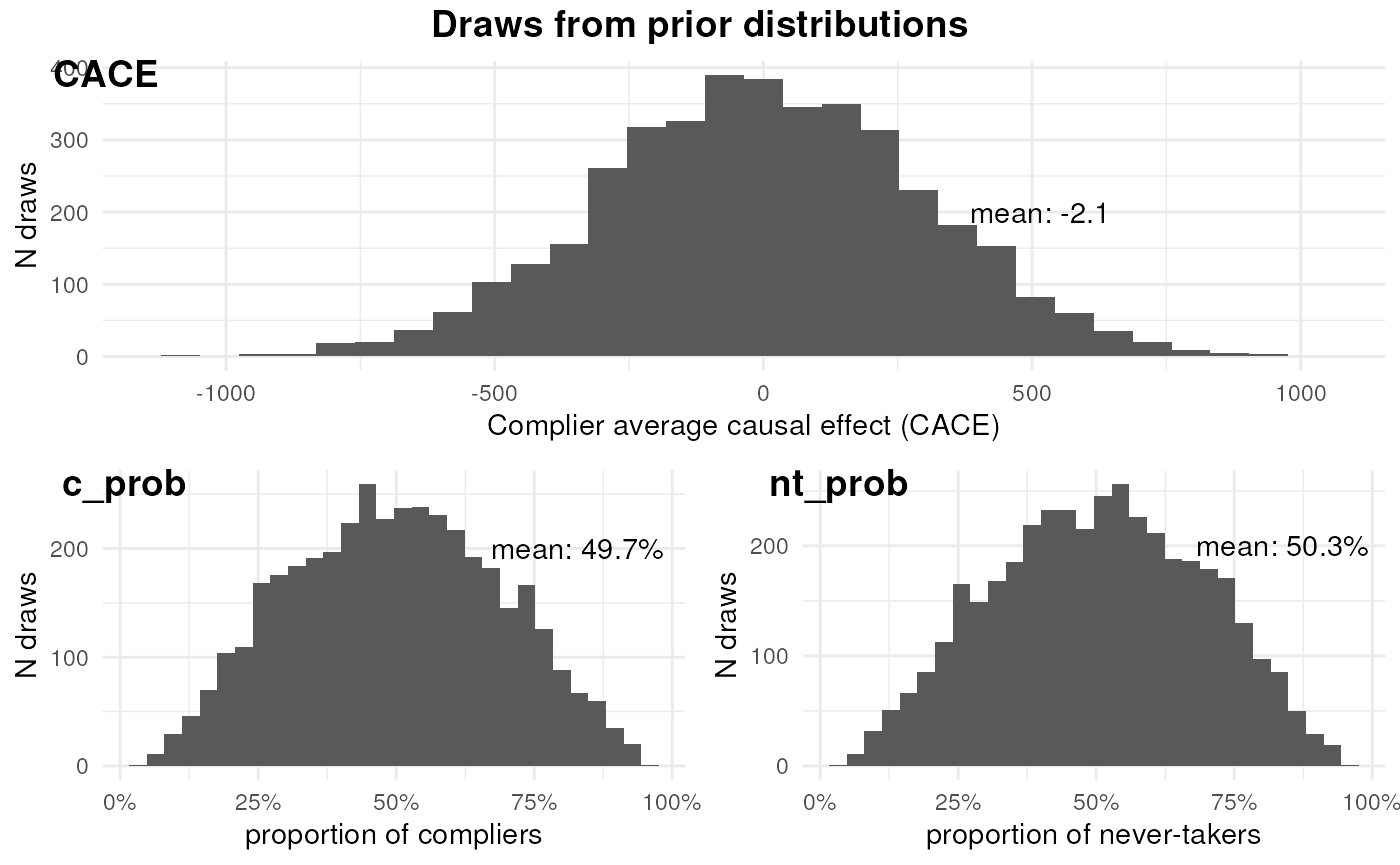
The effect of the feature among compliers is negligible by priors. The proportion of compliers and never-takers are half and half.
Fitting a BIVA model to the data
Now we fit a BIVA model to the data.
ivobj <- biva$new(
  data = df, y = "Y", d = "D", z = "Z",
  x_ymodel = c("X"),
  x_smodel = c("X"),
  ER = 1,
  side = 1,
  beta_mean_ymodel = cbind(rep(5000, 3), rep(0, 3)),
  beta_sd_ymodel = cbind(rep(200, 3), rep(200, 3)),
  beta_mean_smodel = matrix(0, 1, 2),
  beta_sd_smodel = matrix(1, 1, 2),
  sigma_shape_ymodel = rep(1, 3),
  sigma_scale_ymodel = rep(1, 3),
  fit = TRUE
)
#>
#> SAMPLING FOR MODEL 'Gaussian' NOW (CHAIN 1).
#> Chain 1:
#> Chain 1: Gradient evaluation took 5e-06 seconds
#> Chain 1: 1000 transitions using 10 leapfrog steps per transition would take 0.05 seconds.
#> Chain 1: Adjust your expectations accordingly!
#> Chain 1:
#> Chain 1:
#> Chain 1: Iteration:    1 / 2000 [  0%]  (Warmup)
#> Chain 1: Iteration:  200 / 2000 [ 10%]  (Warmup)
#> Chain 1: Iteration:  400 / 2000 [ 20%]  (Warmup)
#> Chain 1: Iteration:  600 / 2000 [ 30%]  (Warmup)
#> Chain 1: Iteration:  800 / 2000 [ 40%]  (Warmup)
#> Chain 1: Iteration: 1000 / 2000 [ 50%]  (Warmup)
#> Chain 1: Iteration: 1001 / 2000 [ 50%]  (Sampling)
#> Chain 1: Iteration: 1200 / 2000 [ 60%]  (Sampling)
#> Chain 1: Iteration: 1400 / 2000 [ 70%]  (Sampling)
#> Chain 1: Iteration: 1600 / 2000 [ 80%]  (Sampling)
#> Chain 1: Iteration: 1800 / 2000 [ 90%]  (Sampling)
#> Chain 1: Iteration: 2000 / 2000 [100%]  (Sampling)
#> Chain 1:
#> Chain 1:  Elapsed Time: 0.217 seconds (Warm-up)
#> Chain 1:                0.089 seconds (Sampling)
#> Chain 1:                0.306 seconds (Total)
#> Chain 1:
#>
#> SAMPLING FOR MODEL 'Gaussian' NOW (CHAIN 2).
#> Chain 2:
#> Chain 2: Gradient evaluation took 3e-06 seconds
#> Chain 2: 1000 transitions using 10 leapfrog steps per transition would take 0.03 seconds.
#> Chain 2: Adjust your expectations accordingly!
#> Chain 2:
#> Chain 2:
#> Chain 2: Iteration:    1 / 2000 [  0%]  (Warmup)
#> Chain 2: Iteration:  200 / 2000 [ 10%]  (Warmup)
#> Chain 2: Iteration:  400 / 2000 [ 20%]  (Warmup)
#> Chain 2: Iteration:  600 / 2000 [ 30%]  (Warmup)
#> Chain 2: Iteration:  800 / 2000 [ 40%]  (Warmup)
#> Chain 2: Iteration: 1000 / 2000 [ 50%]  (Warmup)
#> Chain 2: Iteration: 1001 / 2000 [ 50%]  (Sampling)
#> Chain 2: Iteration: 1200 / 2000 [ 60%]  (Sampling)
#> Chain 2: Iteration: 1400 / 2000 [ 70%]  (Sampling)
#> Chain 2: Iteration: 1600 / 2000 [ 80%]  (Sampling)
#> Chain 2: Iteration: 1800 / 2000 [ 90%]  (Sampling)
#> Chain 2: Iteration: 2000 / 2000 [100%]  (Sampling)
#> Chain 2:
#> Chain 2:  Elapsed Time: 0.202 seconds (Warm-up)
#> Chain 2:                0.074 seconds (Sampling)
#> Chain 2:                0.276 seconds (Total)
#> Chain 2:
#>
#> SAMPLING FOR MODEL 'Gaussian' NOW (CHAIN 3).
#> Chain 3:
#> Chain 3: Gradient evaluation took 5e-06 seconds
#> Chain 3: 1000 transitions using 10 leapfrog steps per transition would take 0.05 seconds.
#> Chain 3: Adjust your expectations accordingly!
#> Chain 3:
#> Chain 3:
#> Chain 3: Iteration:    1 / 2000 [  0%]  (Warmup)
#> Chain 3: Iteration:  200 / 2000 [ 10%]  (Warmup)
#> Chain 3: Iteration:  400 / 2000 [ 20%]  (Warmup)
#> Chain 3: Iteration:  600 / 2000 [ 30%]  (Warmup)
#> Chain 3: Iteration:  800 / 2000 [ 40%]  (Warmup)
#> Chain 3: Iteration: 1000 / 2000 [ 50%]  (Warmup)
#> Chain 3: Iteration: 1001 / 2000 [ 50%]  (Sampling)
#> Chain 3: Iteration: 1200 / 2000 [ 60%]  (Sampling)
#> Chain 3: Iteration: 1400 / 2000 [ 70%]  (Sampling)
#> Chain 3: Iteration: 1600 / 2000 [ 80%]  (Sampling)
#> Chain 3: Iteration: 1800 / 2000 [ 90%]  (Sampling)
#> Chain 3: Iteration: 2000 / 2000 [100%]  (Sampling)
#> Chain 3:
#> Chain 3:  Elapsed Time: 0.233 seconds (Warm-up)
#> Chain 3:                0.07 seconds (Sampling)
#> Chain 3:                0.303 seconds (Total)
#> Chain 3:
#>
#> SAMPLING FOR MODEL 'Gaussian' NOW (CHAIN 4).
#> Chain 4:
#> Chain 4: Gradient evaluation took 4e-06 seconds
#> Chain 4: 1000 transitions using 10 leapfrog steps per transition would take 0.04 seconds.
#> Chain 4: Adjust your expectations accordingly!
#> Chain 4:
#> Chain 4:
#> Chain 4: Iteration:    1 / 2000 [  0%]  (Warmup)
#> Chain 4: Iteration:  200 / 2000 [ 10%]  (Warmup)
#> Chain 4: Iteration:  400 / 2000 [ 20%]  (Warmup)
#> Chain 4: Iteration:  600 / 2000 [ 30%]  (Warmup)
#> Chain 4: Iteration:  800 / 2000 [ 40%]  (Warmup)
#> Chain 4: Iteration: 1000 / 2000 [ 50%]  (Warmup)
#> Chain 4: Iteration: 1001 / 2000 [ 50%]  (Sampling)
#> Chain 4: Iteration: 1200 / 2000 [ 60%]  (Sampling)
#> Chain 4: Iteration: 1400 / 2000 [ 70%]  (Sampling)
#> Chain 4: Iteration: 1600 / 2000 [ 80%]  (Sampling)
#> Chain 4: Iteration: 1800 / 2000 [ 90%]  (Sampling)
#> Chain 4: Iteration: 2000 / 2000 [100%]  (Sampling)
#> Chain 4:
#> Chain 4:  Elapsed Time: 0.2 seconds (Warm-up)
#> Chain 4:                0.074 seconds (Sampling)
#> Chain 4:                0.274 seconds (Total)
#> Chain 4:
#> Fitting model to the data
#>
#> SAMPLING FOR MODEL 'Gaussian' NOW (CHAIN 1).
#> Chain 1:
#> Chain 1: Gradient evaluation took 0.0002 seconds
#> Chain 1: 1000 transitions using 10 leapfrog steps per transition would take 2 seconds.
#> Chain 1: Adjust your expectations accordingly!
#> Chain 1:
#> Chain 1:
#> Chain 1: Iteration:    1 / 2000 [  0%]  (Warmup)
#> Chain 1: Iteration:  200 / 2000 [ 10%]  (Warmup)
#> Chain 1: Iteration:  400 / 2000 [ 20%]  (Warmup)
#> Chain 1: Iteration:  600 / 2000 [ 30%]  (Warmup)
#> Chain 1: Iteration:  800 / 2000 [ 40%]  (Warmup)
#> Chain 1: Iteration: 1000 / 2000 [ 50%]  (Warmup)
#> Chain 1: Iteration: 1001 / 2000 [ 50%]  (Sampling)
#> Chain 1: Iteration: 1200 / 2000 [ 60%]  (Sampling)
#> Chain 1: Iteration: 1400 / 2000 [ 70%]  (Sampling)
#> Chain 1: Iteration: 1600 / 2000 [ 80%]  (Sampling)
#> Chain 1: Iteration: 1800 / 2000 [ 90%]  (Sampling)
#> Chain 1: Iteration: 2000 / 2000 [100%]  (Sampling)
#> Chain 1:
#> Chain 1:  Elapsed Time: 12.439 seconds (Warm-up)
#> Chain 1:                1.284 seconds (Sampling)
#> Chain 1:                13.723 seconds (Total)
#> Chain 1:
#>
#> SAMPLING FOR MODEL 'Gaussian' NOW (CHAIN 2).
#> Chain 2:
#> Chain 2: Gradient evaluation took 0.000159 seconds
#> Chain 2: 1000 transitions using 10 leapfrog steps per transition would take 1.59 seconds.
#> Chain 2: Adjust your expectations accordingly!
#> Chain 2:
#> Chain 2:
#> Chain 2: Iteration:    1 / 2000 [  0%]  (Warmup)
#> Chain 2: Iteration:  200 / 2000 [ 10%]  (Warmup)
#> Chain 2: Iteration:  400 / 2000 [ 20%]  (Warmup)
#> Chain 2: Iteration:  600 / 2000 [ 30%]  (Warmup)
#> Chain 2: Iteration:  800 / 2000 [ 40%]  (Warmup)
#> Chain 2: Iteration: 1000 / 2000 [ 50%]  (Warmup)
#> Chain 2: Iteration: 1001 / 2000 [ 50%]  (Sampling)
#> Chain 2: Iteration: 1200 / 2000 [ 60%]  (Sampling)
#> Chain 2: Iteration: 1400 / 2000 [ 70%]  (Sampling)
#> Chain 2: Iteration: 1600 / 2000 [ 80%]  (Sampling)
#> Chain 2: Iteration: 1800 / 2000 [ 90%]  (Sampling)
#> Chain 2: Iteration: 2000 / 2000 [100%]  (Sampling)
#> Chain 2:
#> Chain 2:  Elapsed Time: 12.948 seconds (Warm-up)
#> Chain 2:                1.286 seconds (Sampling)
#> Chain 2:                14.234 seconds (Total)
#> Chain 2:
#>
#> SAMPLING FOR MODEL 'Gaussian' NOW (CHAIN 3).
#> Chain 3:
#> Chain 3: Gradient evaluation took 0.000175 seconds
#> Chain 3: 1000 transitions using 10 leapfrog steps per transition would take 1.75 seconds.
#> Chain 3: Adjust your expectations accordingly!
#> Chain 3:
#> Chain 3:
#> Chain 3: Iteration:    1 / 2000 [  0%]  (Warmup)
#> Chain 3: Iteration:  200 / 2000 [ 10%]  (Warmup)
#> Chain 3: Iteration:  400 / 2000 [ 20%]  (Warmup)
#> Chain 3: Iteration:  600 / 2000 [ 30%]  (Warmup)
#> Chain 3: Iteration:  800 / 2000 [ 40%]  (Warmup)
#> Chain 3: Iteration: 1000 / 2000 [ 50%]  (Warmup)
#> Chain 3: Iteration: 1001 / 2000 [ 50%]  (Sampling)
#> Chain 3: Iteration: 1200 / 2000 [ 60%]  (Sampling)
#> Chain 3: Iteration: 1400 / 2000 [ 70%]  (Sampling)
#> Chain 3: Iteration: 1600 / 2000 [ 80%]  (Sampling)
#> Chain 3: Iteration: 1800 / 2000 [ 90%]  (Sampling)
#> Chain 3: Iteration: 2000 / 2000 [100%]  (Sampling)
#> Chain 3:
#> Chain 3:  Elapsed Time: 13.689 seconds (Warm-up)
#> Chain 3:                1.25 seconds (Sampling)
#> Chain 3:                14.939 seconds (Total)
#> Chain 3:
#>
#> SAMPLING FOR MODEL 'Gaussian' NOW (CHAIN 4).
#> Chain 4:
#> Chain 4: Gradient evaluation took 0.000158 seconds
#> Chain 4: 1000 transitions using 10 leapfrog steps per transition would take 1.58 seconds.
#> Chain 4: Adjust your expectations accordingly!
#> Chain 4:
#> Chain 4:
#> Chain 4: Iteration:    1 / 2000 [  0%]  (Warmup)
#> Chain 4: Iteration:  200 / 2000 [ 10%]  (Warmup)
#> Chain 4: Iteration:  400 / 2000 [ 20%]  (Warmup)
#> Chain 4: Iteration:  600 / 2000 [ 30%]  (Warmup)
#> Chain 4: Iteration:  800 / 2000 [ 40%]  (Warmup)
#> Chain 4: Iteration: 1000 / 2000 [ 50%]  (Warmup)
#> Chain 4: Iteration: 1001 / 2000 [ 50%]  (Sampling)
#> Chain 4: Iteration: 1200 / 2000 [ 60%]  (Sampling)
#> Chain 4: Iteration: 1400 / 2000 [ 70%]  (Sampling)
#> Chain 4: Iteration: 1600 / 2000 [ 80%]  (Sampling)
#> Chain 4: Iteration: 1800 / 2000 [ 90%]  (Sampling)
#> Chain 4: Iteration: 2000 / 2000 [100%]  (Sampling)
#> Chain 4:
#> Chain 4:  Elapsed Time: 14.098 seconds (Warm-up)
#> Chain 4:                1.295 seconds (Sampling)
#> Chain 4:                15.393 seconds (Total)
#> Chain 4:
#> Found more than one class "Rcpp_rstantools_model_logit" in cache; using the first, from namespace 'biva'
#> Also defined by 'im'
#> Found more than one class "Rcpp_rstantools_model_logit" in cache; using the first, from namespace 'biva'
#> Also defined by 'im'
#> All diagnostics look fine
We can look at the trace plot of outcomes in each strata to see if the chains mixed and converged. The three plots are the posterior draws of the mean outcomes among the compliers assigned to control, the compliers nudged to treatment, and the never-takers.
ivobj$tracePlot()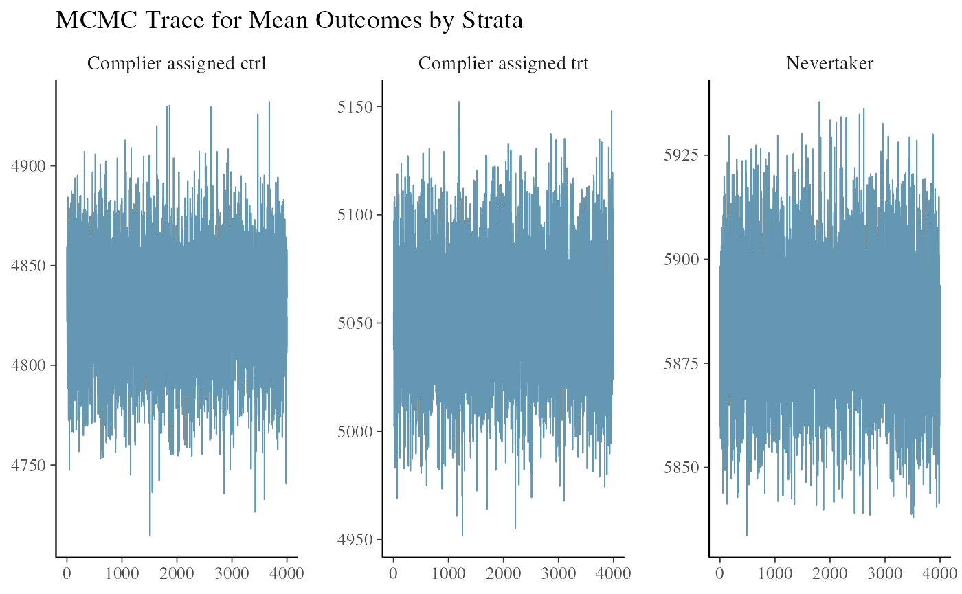
The convergence and mixing look good.
A weak instrument test can be run to understand if there is concern about the estimates due to a low proportion of compliers.
ivobj$weakIVTest()
#> The instrument is not considered weak, resulting in an estimated 41% of compliers in the population.
The proportion of compliers is at a decent level to avoid potential issues. More details are covered in a later example of weak instrument.
We can use the following methods to summarize our findings:
# Posterior distribution of the strata probability
ivobj$strataProbEstimate()
#> Given the data, we estimate that there is a 41% probability that the unit is a complier, and a 59% probability that the unit is a never-taker.
# Posterior probability that CACE is greater than 200
ivobj$calcProb(a = 200)
#> Given the data, we estimate that the probability that the effect is more than 200 is 76%.
# Posterior median of the CACE
ivobj$pointEstimate()
#> [1] 224.8387
# Posterior mean of the CACE
ivobj$pointEstimate(median = FALSE)
#> [1] 224.9999
# 75% credible interval of the CACE
ivobj$credibleInterval()
#> Given the data, we estimate that there is a 75% probability that the CACE is between 183.05 and 267.3.
# 95% credible interval of the CACE
ivobj$credibleInterval(width = 0.95)
#> Given the data, we estimate that there is a 95% probability that the CACE is between 153.14 and 299.06.
The posterior does a good job in recovering the direction and the magnitude of the true impact among compliers. The statement about the probability that the CACE is greater than 200, or with what probability it falls in a certain range, are direct answers to the business question of whether the feature is worth launching. This is prohibited by any frequentist approach where the effect parameter is treated as nonrandom and the confidence interval captures uncertainty in the sampling distribution of data instead of in the parameter itself.
Users can also visualize how the data updates our knowledge about the impact by comparing its posterior distribution with the prior. This can be done by running the following methods. The output are interactive html widgets. The outputs are hidden here.
ivobj$vizdraws(
  display_mode_name = TRUE, breaks = 200,
  break_names = c("< 200", "> 200")
)
ivobj$lollipop(threshold = 200, mediumText = 8)
The same procedures can be applied to a two-side noncompliance setting, which usually happens when the feature has already been launched or the assigned nudge can be leaked.
Demonstration 2: two-side noncompliance
Data simulation
We again simulate some data from a hypothetical randomized experiment with noncompliance. Now we want to evaluate the impact of the feature after it is launched. In this case, we have two-side noncompliance where the assigned treated units can opt out and the assigned control can opt in.
Therefore, there are 3 principal strata: compliers, never-takers, and always-takers.
set.seed(1997)
n <- 200

# Covariates
# X (continuous, observed)
# U (binary, unobserved)
X <- rnorm(n)
U <- rbinom(n, 1, 0.5)

## True memberships of principal strata (1:c,2:nt,3:at): S-model depends only on U
true.PS <- rep(0, n)
U1.ind <- (U == 1)
U0.ind <- (U == 0)
num.U1 <- sum(U1.ind)
num.U0 <- sum(U0.ind)
true.PS[U1.ind] <- t(rmultinom(num.U1, 1, c(0.6, 0.3, 0.1))) %*% c(1, 2, 3)
true.PS[U0.ind] <- t(rmultinom(num.U0, 1, c(0.4, 0.5, 0.1))) %*% c(1, 2, 3)

## Treatment assigned: half control & half treatment
Z <- c(rep(0, n / 2), rep(1, n / 2))

## Treatment received: determined by principal strata and treatment assigned
D <- rep(0, n)
c.trt.ind <- (true.PS == 1) & (Z == 1)
c.ctrl.ind <- (true.PS == 1) & (Z == 0)
nt.ind <- (true.PS == 2)
at.ind <- (true.PS == 3)
num.c.trt <- sum(c.trt.ind)
num.c.ctrl <- sum(c.ctrl.ind)
num.nt <- sum(nt.ind)
num.at <- sum(at.ind)
D[at.ind] <- rep(1, num.at)
D[c.trt.ind] <- rep(1, num.c.trt)

## Generate observed outcome: Y-model depend on X, U, D, and principal strata
Y <- rep(0, n)
Y[c.ctrl.ind] <- rnorm(num.c.ctrl,
  mean = 5000 + 100 * X[c.ctrl.ind] - 300 * U[c.ctrl.ind],
  sd = 50
)
Y[c.trt.ind] <- rnorm(num.c.trt,
  mean = 5250 + 100 * X[c.trt.ind] - 300 * U[c.trt.ind],
  sd = 50
)
Y[nt.ind] <- rnorm(num.nt,
  mean = 6000 + 100 * X[nt.ind] - 300 * U[nt.ind],
  sd = 50
)
Y[at.ind] <- rnorm(num.at,
  mean = 4500 + 100 * X[at.ind] - 300 * U[at.ind],
  sd = 50
)


df <- data.frame(Y = Y, Z = Z, D = D, X = X, U = U)
With always-takers, some changes are applied to the data-generating process. For the strata model, when U = 1, a unit is a complier, a never-taker, or an always-taker with probability 0.6, 0.3, and 0.1, respectively. When U = 0, a unit is a complier, a never-taker, or an always-taker with probability 0.4, 0.5, and 0.1, respectively.
The always-takers will always adopt the treatment feature. With exclusion restriction, we add one outcome model for always-takers. The remaining models are kept the same. The CACE of the feature is still 5250 - 5000 = 250.
OLS analysis
We again fit an OLS model with the adopted treatment D and the observed covariate X to see the caveats.
OLS <- lm(data = df, formula = Y ~ D + X)
summary(OLS)
#>
#> Call:
#> lm(formula = Y ~ D + X, data = df)
#>
#> Residuals:
#>    Min     1Q Median     3Q    Max
#> -943.3 -502.1  171.7  410.2  553.0
#>
#> Coefficients:
#>             Estimate Std. Error t value Pr(>|t|)
#> (Intercept)  5530.36      43.13 128.216  < 2e-16 ***
#> D            -628.11      71.47  -8.788 7.49e-16 ***
#> X             108.69      34.45   3.154  0.00186 **
#> ---
#> Signif. codes:  0 '***' 0.001 '**' 0.01 '*' 0.05 '.' 0.1 ' ' 1
#>
#> Residual standard error: 485 on 197 degrees of freedom
#> Multiple R-squared:  0.303,  Adjusted R-squared:  0.2959
#> F-statistic: 42.81 on 2 and 197 DF,  p-value: 3.634e-16
confint(OLS, "D")
#>       2.5 %    97.5 %
#> D -769.0591 -487.1565
It returns misleading significant results again.
We restart the BIVA workflow to fix this issue.
Prior predictive checking
With two-side noncompliance, we set side = 2. The number of models in specifying priors should be updated as well.
ivobj <- biva$new(
  data = df, y = "Y", d = "D", z = "Z",
  x_ymodel = c("X"),
  x_smodel = c("X"),
  ER = 1,
  side = 2,
  beta_mean_ymodel = cbind(rep(5000, 4), rep(0, 4)),
  beta_sd_ymodel = cbind(rep(200, 4), rep(200, 4)),
  beta_mean_smodel = matrix(0, 2, 2),
  beta_sd_smodel = matrix(1, 2, 2),
  sigma_shape_ymodel = rep(1, 4),
  sigma_scale_ymodel = rep(1, 4),
  fit = FALSE
)
#>
#> SAMPLING FOR MODEL 'Gaussian' NOW (CHAIN 1).
#> Chain 1:
#> Chain 1: Gradient evaluation took 5e-06 seconds
#> Chain 1: 1000 transitions using 10 leapfrog steps per transition would take 0.05 seconds.
#> Chain 1: Adjust your expectations accordingly!
#> Chain 1:
#> Chain 1:
#> Chain 1: Iteration:    1 / 2000 [  0%]  (Warmup)
#> Chain 1: Iteration:  200 / 2000 [ 10%]  (Warmup)
#> Chain 1: Iteration:  400 / 2000 [ 20%]  (Warmup)
#> Chain 1: Iteration:  600 / 2000 [ 30%]  (Warmup)
#> Chain 1: Iteration:  800 / 2000 [ 40%]  (Warmup)
#> Chain 1: Iteration: 1000 / 2000 [ 50%]  (Warmup)
#> Chain 1: Iteration: 1001 / 2000 [ 50%]  (Sampling)
#> Chain 1: Iteration: 1200 / 2000 [ 60%]  (Sampling)
#> Chain 1: Iteration: 1400 / 2000 [ 70%]  (Sampling)
#> Chain 1: Iteration: 1600 / 2000 [ 80%]  (Sampling)
#> Chain 1: Iteration: 1800 / 2000 [ 90%]  (Sampling)
#> Chain 1: Iteration: 2000 / 2000 [100%]  (Sampling)
#> Chain 1:
#> Chain 1:  Elapsed Time: 0.302 seconds (Warm-up)
#> Chain 1:                0.084 seconds (Sampling)
#> Chain 1:                0.386 seconds (Total)
#> Chain 1:
#>
#> SAMPLING FOR MODEL 'Gaussian' NOW (CHAIN 2).
#> Chain 2:
#> Chain 2: Gradient evaluation took 4e-06 seconds
#> Chain 2: 1000 transitions using 10 leapfrog steps per transition would take 0.04 seconds.
#> Chain 2: Adjust your expectations accordingly!
#> Chain 2:
#> Chain 2:
#> Chain 2: Iteration:    1 / 2000 [  0%]  (Warmup)
#> Chain 2: Iteration:  200 / 2000 [ 10%]  (Warmup)
#> Chain 2: Iteration:  400 / 2000 [ 20%]  (Warmup)
#> Chain 2: Iteration:  600 / 2000 [ 30%]  (Warmup)
#> Chain 2: Iteration:  800 / 2000 [ 40%]  (Warmup)
#> Chain 2: Iteration: 1000 / 2000 [ 50%]  (Warmup)
#> Chain 2: Iteration: 1001 / 2000 [ 50%]  (Sampling)
#> Chain 2: Iteration: 1200 / 2000 [ 60%]  (Sampling)
#> Chain 2: Iteration: 1400 / 2000 [ 70%]  (Sampling)
#> Chain 2: Iteration: 1600 / 2000 [ 80%]  (Sampling)
#> Chain 2: Iteration: 1800 / 2000 [ 90%]  (Sampling)
#> Chain 2: Iteration: 2000 / 2000 [100%]  (Sampling)
#> Chain 2:
#> Chain 2:  Elapsed Time: 0.285 seconds (Warm-up)
#> Chain 2:                0.092 seconds (Sampling)
#> Chain 2:                0.377 seconds (Total)
#> Chain 2:
#>
#> SAMPLING FOR MODEL 'Gaussian' NOW (CHAIN 3).
#> Chain 3:
#> Chain 3: Gradient evaluation took 4e-06 seconds
#> Chain 3: 1000 transitions using 10 leapfrog steps per transition would take 0.04 seconds.
#> Chain 3: Adjust your expectations accordingly!
#> Chain 3:
#> Chain 3:
#> Chain 3: Iteration:    1 / 2000 [  0%]  (Warmup)
#> Chain 3: Iteration:  200 / 2000 [ 10%]  (Warmup)
#> Chain 3: Iteration:  400 / 2000 [ 20%]  (Warmup)
#> Chain 3: Iteration:  600 / 2000 [ 30%]  (Warmup)
#> Chain 3: Iteration:  800 / 2000 [ 40%]  (Warmup)
#> Chain 3: Iteration: 1000 / 2000 [ 50%]  (Warmup)
#> Chain 3: Iteration: 1001 / 2000 [ 50%]  (Sampling)
#> Chain 3: Iteration: 1200 / 2000 [ 60%]  (Sampling)
#> Chain 3: Iteration: 1400 / 2000 [ 70%]  (Sampling)
#> Chain 3: Iteration: 1600 / 2000 [ 80%]  (Sampling)
#> Chain 3: Iteration: 1800 / 2000 [ 90%]  (Sampling)
#> Chain 3: Iteration: 2000 / 2000 [100%]  (Sampling)
#> Chain 3:
#> Chain 3:  Elapsed Time: 0.296 seconds (Warm-up)
#> Chain 3:                0.088 seconds (Sampling)
#> Chain 3:                0.384 seconds (Total)
#> Chain 3:
#>
#> SAMPLING FOR MODEL 'Gaussian' NOW (CHAIN 4).
#> Chain 4:
#> Chain 4: Gradient evaluation took 4e-06 seconds
#> Chain 4: 1000 transitions using 10 leapfrog steps per transition would take 0.04 seconds.
#> Chain 4: Adjust your expectations accordingly!
#> Chain 4:
#> Chain 4:
#> Chain 4: Iteration:    1 / 2000 [  0%]  (Warmup)
#> Chain 4: Iteration:  200 / 2000 [ 10%]  (Warmup)
#> Chain 4: Iteration:  400 / 2000 [ 20%]  (Warmup)
#> Chain 4: Iteration:  600 / 2000 [ 30%]  (Warmup)
#> Chain 4: Iteration:  800 / 2000 [ 40%]  (Warmup)
#> Chain 4: Iteration: 1000 / 2000 [ 50%]  (Warmup)
#> Chain 4: Iteration: 1001 / 2000 [ 50%]  (Sampling)
#> Chain 4: Iteration: 1200 / 2000 [ 60%]  (Sampling)
#> Chain 4: Iteration: 1400 / 2000 [ 70%]  (Sampling)
#> Chain 4: Iteration: 1600 / 2000 [ 80%]  (Sampling)
#> Chain 4: Iteration: 1800 / 2000 [ 90%]  (Sampling)
#> Chain 4: Iteration: 2000 / 2000 [100%]  (Sampling)
#> Chain 4:
#> Chain 4:  Elapsed Time: 0.309 seconds (Warm-up)
#> Chain 4:                0.086 seconds (Sampling)
#> Chain 4:                0.395 seconds (Total)
#> Chain 4:

ivobj$plotPrior()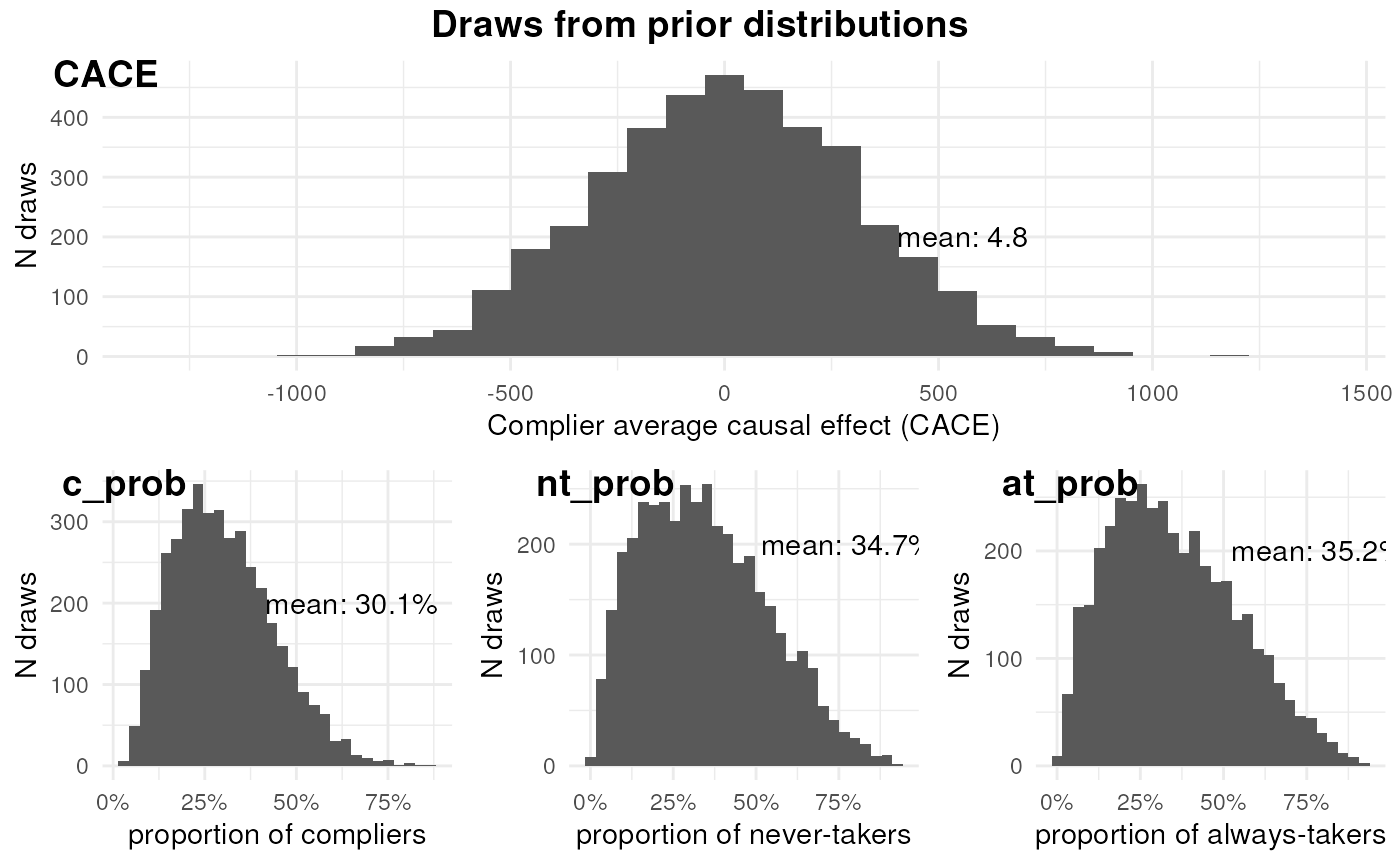
The effect of the feature among compliers is negligible. The proportions of compliers, never-takers, and always-takers are similar.
Fitting a BIVA model to the data
Now we fit a BIVA model to the data.
ivobj <- biva$new(
  data = df, y = "Y", d = "D", z = "Z",
  x_ymodel = c("X"),
  x_smodel = c("X"),
  ER = 1,
  side = 2,
  beta_mean_ymodel = cbind(rep(5000, 4), rep(0, 4)),
  beta_sd_ymodel = cbind(rep(200, 4), rep(200, 4)),
  beta_mean_smodel = matrix(0, 2, 2),
  beta_sd_smodel = matrix(1, 2, 2),
  sigma_shape_ymodel = rep(1, 4),
  sigma_scale_ymodel = rep(1, 4),
  fit = TRUE
)
#>
#> SAMPLING FOR MODEL 'Gaussian' NOW (CHAIN 1).
#> Chain 1:
#> Chain 1: Gradient evaluation took 5e-06 seconds
#> Chain 1: 1000 transitions using 10 leapfrog steps per transition would take 0.05 seconds.
#> Chain 1: Adjust your expectations accordingly!
#> Chain 1:
#> Chain 1:
#> Chain 1: Iteration:    1 / 2000 [  0%]  (Warmup)
#> Chain 1: Iteration:  200 / 2000 [ 10%]  (Warmup)
#> Chain 1: Iteration:  400 / 2000 [ 20%]  (Warmup)
#> Chain 1: Iteration:  600 / 2000 [ 30%]  (Warmup)
#> Chain 1: Iteration:  800 / 2000 [ 40%]  (Warmup)
#> Chain 1: Iteration: 1000 / 2000 [ 50%]  (Warmup)
#> Chain 1: Iteration: 1001 / 2000 [ 50%]  (Sampling)
#> Chain 1: Iteration: 1200 / 2000 [ 60%]  (Sampling)
#> Chain 1: Iteration: 1400 / 2000 [ 70%]  (Sampling)
#> Chain 1: Iteration: 1600 / 2000 [ 80%]  (Sampling)
#> Chain 1: Iteration: 1800 / 2000 [ 90%]  (Sampling)
#> Chain 1: Iteration: 2000 / 2000 [100%]  (Sampling)
#> Chain 1:
#> Chain 1:  Elapsed Time: 0.305 seconds (Warm-up)
#> Chain 1:                0.088 seconds (Sampling)
#> Chain 1:                0.393 seconds (Total)
#> Chain 1:
#>
#> SAMPLING FOR MODEL 'Gaussian' NOW (CHAIN 2).
#> Chain 2:
#> Chain 2: Gradient evaluation took 4e-06 seconds
#> Chain 2: 1000 transitions using 10 leapfrog steps per transition would take 0.04 seconds.
#> Chain 2: Adjust your expectations accordingly!
#> Chain 2:
#> Chain 2:
#> Chain 2: Iteration:    1 / 2000 [  0%]  (Warmup)
#> Chain 2: Iteration:  200 / 2000 [ 10%]  (Warmup)
#> Chain 2: Iteration:  400 / 2000 [ 20%]  (Warmup)
#> Chain 2: Iteration:  600 / 2000 [ 30%]  (Warmup)
#> Chain 2: Iteration:  800 / 2000 [ 40%]  (Warmup)
#> Chain 2: Iteration: 1000 / 2000 [ 50%]  (Warmup)
#> Chain 2: Iteration: 1001 / 2000 [ 50%]  (Sampling)
#> Chain 2: Iteration: 1200 / 2000 [ 60%]  (Sampling)
#> Chain 2: Iteration: 1400 / 2000 [ 70%]  (Sampling)
#> Chain 2: Iteration: 1600 / 2000 [ 80%]  (Sampling)
#> Chain 2: Iteration: 1800 / 2000 [ 90%]  (Sampling)
#> Chain 2: Iteration: 2000 / 2000 [100%]  (Sampling)
#> Chain 2:
#> Chain 2:  Elapsed Time: 0.342 seconds (Warm-up)
#> Chain 2:                0.086 seconds (Sampling)
#> Chain 2:                0.428 seconds (Total)
#> Chain 2:
#>
#> SAMPLING FOR MODEL 'Gaussian' NOW (CHAIN 3).
#> Chain 3:
#> Chain 3: Gradient evaluation took 4e-06 seconds
#> Chain 3: 1000 transitions using 10 leapfrog steps per transition would take 0.04 seconds.
#> Chain 3: Adjust your expectations accordingly!
#> Chain 3:
#> Chain 3:
#> Chain 3: Iteration:    1 / 2000 [  0%]  (Warmup)
#> Chain 3: Iteration:  200 / 2000 [ 10%]  (Warmup)
#> Chain 3: Iteration:  400 / 2000 [ 20%]  (Warmup)
#> Chain 3: Iteration:  600 / 2000 [ 30%]  (Warmup)
#> Chain 3: Iteration:  800 / 2000 [ 40%]  (Warmup)
#> Chain 3: Iteration: 1000 / 2000 [ 50%]  (Warmup)
#> Chain 3: Iteration: 1001 / 2000 [ 50%]  (Sampling)
#> Chain 3: Iteration: 1200 / 2000 [ 60%]  (Sampling)
#> Chain 3: Iteration: 1400 / 2000 [ 70%]  (Sampling)
#> Chain 3: Iteration: 1600 / 2000 [ 80%]  (Sampling)
#> Chain 3: Iteration: 1800 / 2000 [ 90%]  (Sampling)
#> Chain 3: Iteration: 2000 / 2000 [100%]  (Sampling)
#> Chain 3:
#> Chain 3:  Elapsed Time: 0.309 seconds (Warm-up)
#> Chain 3:                0.09 seconds (Sampling)
#> Chain 3:                0.399 seconds (Total)
#> Chain 3:
#>
#> SAMPLING FOR MODEL 'Gaussian' NOW (CHAIN 4).
#> Chain 4:
#> Chain 4: Gradient evaluation took 4e-06 seconds
#> Chain 4: 1000 transitions using 10 leapfrog steps per transition would take 0.04 seconds.
#> Chain 4: Adjust your expectations accordingly!
#> Chain 4:
#> Chain 4:
#> Chain 4: Iteration:    1 / 2000 [  0%]  (Warmup)
#> Chain 4: Iteration:  200 / 2000 [ 10%]  (Warmup)
#> Chain 4: Iteration:  400 / 2000 [ 20%]  (Warmup)
#> Chain 4: Iteration:  600 / 2000 [ 30%]  (Warmup)
#> Chain 4: Iteration:  800 / 2000 [ 40%]  (Warmup)
#> Chain 4: Iteration: 1000 / 2000 [ 50%]  (Warmup)
#> Chain 4: Iteration: 1001 / 2000 [ 50%]  (Sampling)
#> Chain 4: Iteration: 1200 / 2000 [ 60%]  (Sampling)
#> Chain 4: Iteration: 1400 / 2000 [ 70%]  (Sampling)
#> Chain 4: Iteration: 1600 / 2000 [ 80%]  (Sampling)
#> Chain 4: Iteration: 1800 / 2000 [ 90%]  (Sampling)
#> Chain 4: Iteration: 2000 / 2000 [100%]  (Sampling)
#> Chain 4:
#> Chain 4:  Elapsed Time: 0.314 seconds (Warm-up)
#> Chain 4:                0.088 seconds (Sampling)
#> Chain 4:                0.402 seconds (Total)
#> Chain 4:
#> Fitting model to the data
#>
#> SAMPLING FOR MODEL 'Gaussian' NOW (CHAIN 1).
#> Chain 1:
#> Chain 1: Gradient evaluation took 0.0002 seconds
#> Chain 1: 1000 transitions using 10 leapfrog steps per transition would take 2 seconds.
#> Chain 1: Adjust your expectations accordingly!
#> Chain 1:
#> Chain 1:
#> Chain 1: Iteration:    1 / 2000 [  0%]  (Warmup)
#> Chain 1: Iteration:  200 / 2000 [ 10%]  (Warmup)
#> Chain 1: Iteration:  400 / 2000 [ 20%]  (Warmup)
#> Chain 1: Iteration:  600 / 2000 [ 30%]  (Warmup)
#> Chain 1: Iteration:  800 / 2000 [ 40%]  (Warmup)
#> Chain 1: Iteration: 1000 / 2000 [ 50%]  (Warmup)
#> Chain 1: Iteration: 1001 / 2000 [ 50%]  (Sampling)
#> Chain 1: Iteration: 1200 / 2000 [ 60%]  (Sampling)
#> Chain 1: Iteration: 1400 / 2000 [ 70%]  (Sampling)
#> Chain 1: Iteration: 1600 / 2000 [ 80%]  (Sampling)
#> Chain 1: Iteration: 1800 / 2000 [ 90%]  (Sampling)
#> Chain 1: Iteration: 2000 / 2000 [100%]  (Sampling)
#> Chain 1:
#> Chain 1:  Elapsed Time: 49.003 seconds (Warm-up)
#> Chain 1:                1.613 seconds (Sampling)
#> Chain 1:                50.616 seconds (Total)
#> Chain 1:
#>
#> SAMPLING FOR MODEL 'Gaussian' NOW (CHAIN 2).
#> Chain 2:
#> Chain 2: Gradient evaluation took 0.000225 seconds
#> Chain 2: 1000 transitions using 10 leapfrog steps per transition would take 2.25 seconds.
#> Chain 2: Adjust your expectations accordingly!
#> Chain 2:
#> Chain 2:
#> Chain 2: Iteration:    1 / 2000 [  0%]  (Warmup)
#> Chain 2: Iteration:  200 / 2000 [ 10%]  (Warmup)
#> Chain 2: Iteration:  400 / 2000 [ 20%]  (Warmup)
#> Chain 2: Iteration:  600 / 2000 [ 30%]  (Warmup)
#> Chain 2: Iteration:  800 / 2000 [ 40%]  (Warmup)
#> Chain 2: Iteration: 1000 / 2000 [ 50%]  (Warmup)
#> Chain 2: Iteration: 1001 / 2000 [ 50%]  (Sampling)
#> Chain 2: Iteration: 1200 / 2000 [ 60%]  (Sampling)
#> Chain 2: Iteration: 1400 / 2000 [ 70%]  (Sampling)
#> Chain 2: Iteration: 1600 / 2000 [ 80%]  (Sampling)
#> Chain 2: Iteration: 1800 / 2000 [ 90%]  (Sampling)
#> Chain 2: Iteration: 2000 / 2000 [100%]  (Sampling)
#> Chain 2:
#> Chain 2:  Elapsed Time: 19.432 seconds (Warm-up)
#> Chain 2:                1.614 seconds (Sampling)
#> Chain 2:                21.046 seconds (Total)
#> Chain 2:
#>
#> SAMPLING FOR MODEL 'Gaussian' NOW (CHAIN 3).
#> Chain 3:
#> Chain 3: Gradient evaluation took 0.000205 seconds
#> Chain 3: 1000 transitions using 10 leapfrog steps per transition would take 2.05 seconds.
#> Chain 3: Adjust your expectations accordingly!
#> Chain 3:
#> Chain 3:
#> Chain 3: Iteration:    1 / 2000 [  0%]  (Warmup)
#> Chain 3: Iteration:  200 / 2000 [ 10%]  (Warmup)
#> Chain 3: Iteration:  400 / 2000 [ 20%]  (Warmup)
#> Chain 3: Iteration:  600 / 2000 [ 30%]  (Warmup)
#> Chain 3: Iteration:  800 / 2000 [ 40%]  (Warmup)
#> Chain 3: Iteration: 1000 / 2000 [ 50%]  (Warmup)
#> Chain 3: Iteration: 1001 / 2000 [ 50%]  (Sampling)
#> Chain 3: Iteration: 1200 / 2000 [ 60%]  (Sampling)
#> Chain 3: Iteration: 1400 / 2000 [ 70%]  (Sampling)
#> Chain 3: Iteration: 1600 / 2000 [ 80%]  (Sampling)
#> Chain 3: Iteration: 1800 / 2000 [ 90%]  (Sampling)
#> Chain 3: Iteration: 2000 / 2000 [100%]  (Sampling)
#> Chain 3:
#> Chain 3:  Elapsed Time: 15.769 seconds (Warm-up)
#> Chain 3:                1.633 seconds (Sampling)
#> Chain 3:                17.402 seconds (Total)
#> Chain 3:
#>
#> SAMPLING FOR MODEL 'Gaussian' NOW (CHAIN 4).
#> Chain 4:
#> Chain 4: Gradient evaluation took 0.000196 seconds
#> Chain 4: 1000 transitions using 10 leapfrog steps per transition would take 1.96 seconds.
#> Chain 4: Adjust your expectations accordingly!
#> Chain 4:
#> Chain 4:
#> Chain 4: Iteration:    1 / 2000 [  0%]  (Warmup)
#> Chain 4: Iteration:  200 / 2000 [ 10%]  (Warmup)
#> Chain 4: Iteration:  400 / 2000 [ 20%]  (Warmup)
#> Chain 4: Iteration:  600 / 2000 [ 30%]  (Warmup)
#> Chain 4: Iteration:  800 / 2000 [ 40%]  (Warmup)
#> Chain 4: Iteration: 1000 / 2000 [ 50%]  (Warmup)
#> Chain 4: Iteration: 1001 / 2000 [ 50%]  (Sampling)
#> Chain 4: Iteration: 1200 / 2000 [ 60%]  (Sampling)
#> Chain 4: Iteration: 1400 / 2000 [ 70%]  (Sampling)
#> Chain 4: Iteration: 1600 / 2000 [ 80%]  (Sampling)
#> Chain 4: Iteration: 1800 / 2000 [ 90%]  (Sampling)
#> Chain 4: Iteration: 2000 / 2000 [100%]  (Sampling)
#> Chain 4:
#> Chain 4:  Elapsed Time: 15.827 seconds (Warm-up)
#> Chain 4:                1.643 seconds (Sampling)
#> Chain 4:                17.47 seconds (Total)
#> Chain 4:
#> All diagnostics look fine
We look at the trace plot of outcomes in each strata to see if the chains mixed and converged. The four plots are the posterior draws of the mean outcomes among the compliers assigned to control, the compliers nudged to treatment, the never-takers, and the always-takers.
ivobj$tracePlot()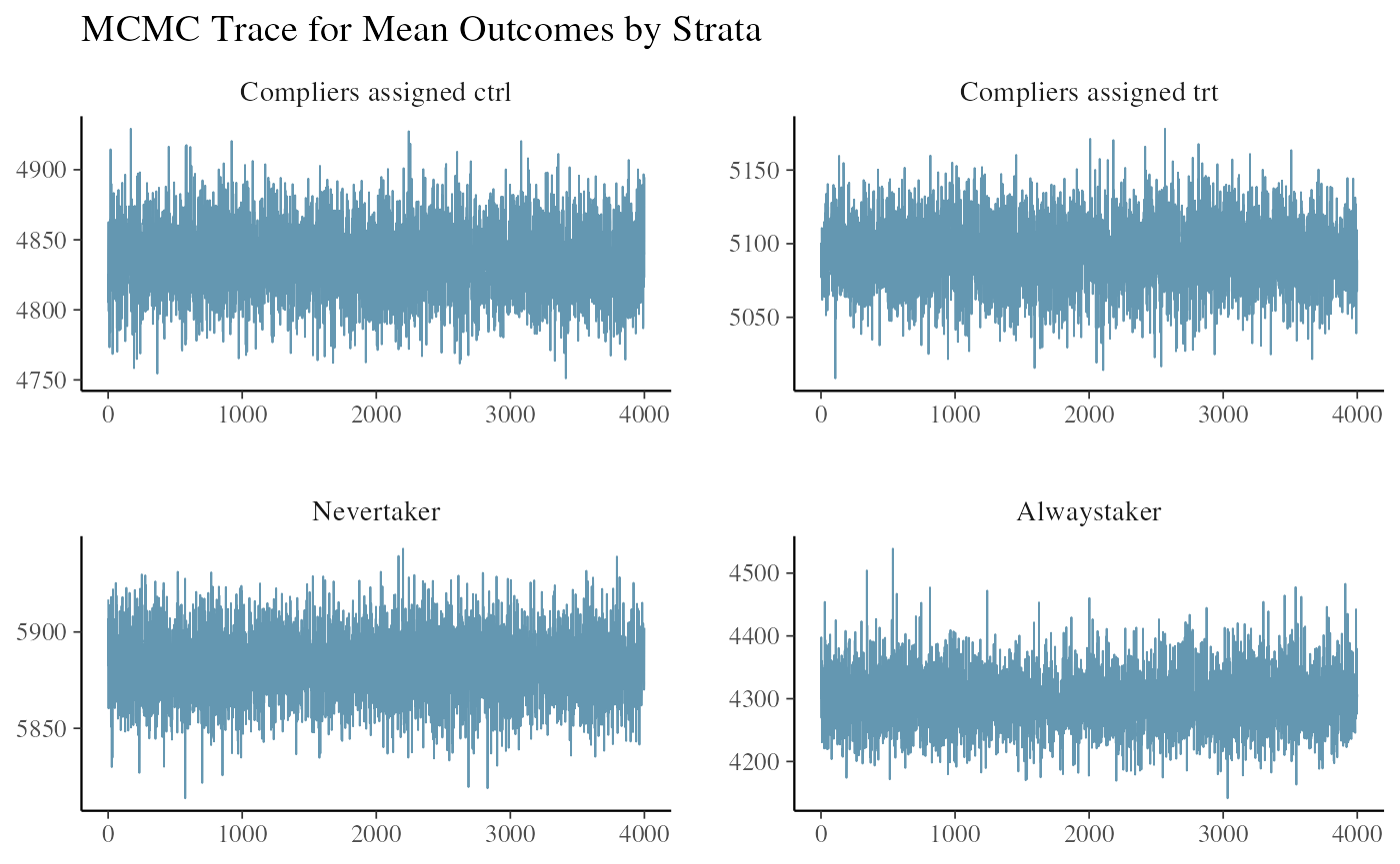
The convergence and mixing look good.
Now we run the weak instrument test.
ivobj$weakIVTest()
#> The instrument is not considered weak, resulting in an estimated 49% of compliers in the population.
No serious concern about weak instrument is found.
We can use the following methods to summarize our findings:
# Posterior distribution of the strata probability
ivobj$strataProbEstimate()
#> Given the data, we estimate that there is a 49% probability that the unit is a complier, a 42% probability that the unit is a never-taker, and a 10% probability that the unit is an always-taker.
# Posterior probability that CACE is greater than 200
ivobj$calcProb(a = 200)
#> Given the data, we estimate that the probability that the effect is more than 200 is 95%.
# Posterior median of the CACE
ivobj$pointEstimate()
#> [1] 258.5116
# Posterior mean of the CACE
ivobj$pointEstimate(median = FALSE)
#> [1] 257.8164
# 75% credible interval of the CACE
ivobj$credibleInterval()
#> Given the data, we estimate that there is a 75% probability that the CACE is between 218.17 and 296.33.
# 95% credible interval of the CACE
ivobj$credibleInterval(width = 0.95)
#> Given the data, we estimate that there is a 95% probability that the CACE is between 188.98 and 324.36.
The posterior returns conclusions close to the ground truth.
Visualizations of how the data updates our knowledge about the impact by comparing its posterior distribution with the prior can be done by running the following methods. We hide these outputs here.
ivobj$vizdraws(
  display_mode_name = TRUE, breaks = 200,
  break_names = c("< 200", "> 200")
)
ivobj$lollipop(threshold = 200, mediumText = 8)
Cautionary note 1: poor mixing of the posterior distribution
The BIVA model essentially fits a mixture likelihood model so it is possible that it predicts incorrectly about the membership of some units to the principal strata. Specifically, in two-side noncompliance, the model may confuse a nudged complier with a always-taker (they both adopt the treatment if assigned to the treatment), or confuse a control complier with a never-taker (they both stay control if assigned to the control). The phenomenon is less common in one-side noncompliance because ruling out the always-takers helps with predicting the compliers, and thus the never-takers. In either case, it is always a good practice to see the trace plot of the posterior distribution immediately after fitting the BIVA model as in the above workflow. It helps with responsible choices of robust metrics for decision-making. Below we show an example.
Data simulation
We simulate some data from the same two-side noncompliance setting as above with a different seed.
set.seed(2001)
n <- 200

# Covariates
# X (continuous, observed)
# U (binary, unobserved)
X <- rnorm(n)
U <- rbinom(n, 1, 0.5)

## True memberships of principal strata (1:c,2:nt,3:at): S-model depends only on U
true.PS <- rep(0, n)
U1.ind <- (U == 1)
U0.ind <- (U == 0)
num.U1 <- sum(U1.ind)
num.U0 <- sum(U0.ind)
true.PS[U1.ind] <- t(rmultinom(num.U1, 1, c(0.6, 0.3, 0.1))) %*% c(1, 2, 3)
true.PS[U0.ind] <- t(rmultinom(num.U0, 1, c(0.4, 0.5, 0.1))) %*% c(1, 2, 3)

## Treatment assigned: half control & half treatment
Z <- c(rep(0, n / 2), rep(1, n / 2))

## Treatment received: determined by principal strata and treatment assigned
D <- rep(0, n)
c.trt.ind <- (true.PS == 1) & (Z == 1)
c.ctrl.ind <- (true.PS == 1) & (Z == 0)
nt.ind <- (true.PS == 2)
at.ind <- (true.PS == 3)
num.c.trt <- sum(c.trt.ind)
num.c.ctrl <- sum(c.ctrl.ind)
num.nt <- sum(nt.ind)
num.at <- sum(at.ind)
D[at.ind] <- rep(1, num.at)
D[c.trt.ind] <- rep(1, num.c.trt)

## Generate observed outcome: Y-model depend on X, U, D, and principal strata
Y <- rep(0, n)
Y[c.ctrl.ind] <- rnorm(num.c.ctrl,
  mean = 5000 + 100 * X[c.ctrl.ind] - 300 * U[c.ctrl.ind],
  sd = 50
)
Y[c.trt.ind] <- rnorm(num.c.trt,
  mean = 5250 + 100 * X[c.trt.ind] - 300 * U[c.trt.ind],
  sd = 50
)
Y[nt.ind] <- rnorm(num.nt,
  mean = 6000 + 100 * X[nt.ind] - 300 * U[nt.ind],
  sd = 50
)
Y[at.ind] <- rnorm(num.at,
  mean = 4500 + 100 * X[at.ind] - 300 * U[at.ind],
  sd = 50
)


df <- data.frame(Y = Y, Z = Z, D = D, X = X, U = U)
Fitting a BIVA model to the data
The prior specifications stay the same so we skip to the step of fitting a BIVA model to the data.
ivobj <- biva$new(
  data = df, y = "Y", d = "D", z = "Z",
  x_ymodel = c("X"),
  x_smodel = c("X"),
  ER = 1,
  side = 2,
  beta_mean_ymodel = cbind(rep(5000, 4), rep(0, 4)),
  beta_sd_ymodel = cbind(rep(200, 4), rep(200, 4)),
  beta_mean_smodel = matrix(0, 2, 2),
  beta_sd_smodel = matrix(1, 2, 2),
  sigma_shape_ymodel = rep(1, 4),
  sigma_scale_ymodel = rep(1, 4),
  fit = TRUE
)
#>
#> SAMPLING FOR MODEL 'Gaussian' NOW (CHAIN 1).
#> Chain 1:
#> Chain 1: Gradient evaluation took 6e-06 seconds
#> Chain 1: 1000 transitions using 10 leapfrog steps per transition would take 0.06 seconds.
#> Chain 1: Adjust your expectations accordingly!
#> Chain 1:
#> Chain 1:
#> Chain 1: Iteration:    1 / 2000 [  0%]  (Warmup)
#> Chain 1: Iteration:  200 / 2000 [ 10%]  (Warmup)
#> Chain 1: Iteration:  400 / 2000 [ 20%]  (Warmup)
#> Chain 1: Iteration:  600 / 2000 [ 30%]  (Warmup)
#> Chain 1: Iteration:  800 / 2000 [ 40%]  (Warmup)
#> Chain 1: Iteration: 1000 / 2000 [ 50%]  (Warmup)
#> Chain 1: Iteration: 1001 / 2000 [ 50%]  (Sampling)
#> Chain 1: Iteration: 1200 / 2000 [ 60%]  (Sampling)
#> Chain 1: Iteration: 1400 / 2000 [ 70%]  (Sampling)
#> Chain 1: Iteration: 1600 / 2000 [ 80%]  (Sampling)
#> Chain 1: Iteration: 1800 / 2000 [ 90%]  (Sampling)
#> Chain 1: Iteration: 2000 / 2000 [100%]  (Sampling)
#> Chain 1:
#> Chain 1:  Elapsed Time: 0.314 seconds (Warm-up)
#> Chain 1:                0.087 seconds (Sampling)
#> Chain 1:                0.401 seconds (Total)
#> Chain 1:
#>
#> SAMPLING FOR MODEL 'Gaussian' NOW (CHAIN 2).
#> Chain 2:
#> Chain 2: Gradient evaluation took 4e-06 seconds
#> Chain 2: 1000 transitions using 10 leapfrog steps per transition would take 0.04 seconds.
#> Chain 2: Adjust your expectations accordingly!
#> Chain 2:
#> Chain 2:
#> Chain 2: Iteration:    1 / 2000 [  0%]  (Warmup)
#> Chain 2: Iteration:  200 / 2000 [ 10%]  (Warmup)
#> Chain 2: Iteration:  400 / 2000 [ 20%]  (Warmup)
#> Chain 2: Iteration:  600 / 2000 [ 30%]  (Warmup)
#> Chain 2: Iteration:  800 / 2000 [ 40%]  (Warmup)
#> Chain 2: Iteration: 1000 / 2000 [ 50%]  (Warmup)
#> Chain 2: Iteration: 1001 / 2000 [ 50%]  (Sampling)
#> Chain 2: Iteration: 1200 / 2000 [ 60%]  (Sampling)
#> Chain 2: Iteration: 1400 / 2000 [ 70%]  (Sampling)
#> Chain 2: Iteration: 1600 / 2000 [ 80%]  (Sampling)
#> Chain 2: Iteration: 1800 / 2000 [ 90%]  (Sampling)
#> Chain 2: Iteration: 2000 / 2000 [100%]  (Sampling)
#> Chain 2:
#> Chain 2:  Elapsed Time: 0.257 seconds (Warm-up)
#> Chain 2:                0.106 seconds (Sampling)
#> Chain 2:                0.363 seconds (Total)
#> Chain 2:
#>
#> SAMPLING FOR MODEL 'Gaussian' NOW (CHAIN 3).
#> Chain 3:
#> Chain 3: Gradient evaluation took 4e-06 seconds
#> Chain 3: 1000 transitions using 10 leapfrog steps per transition would take 0.04 seconds.
#> Chain 3: Adjust your expectations accordingly!
#> Chain 3:
#> Chain 3:
#> Chain 3: Iteration:    1 / 2000 [  0%]  (Warmup)
#> Chain 3: Iteration:  200 / 2000 [ 10%]  (Warmup)
#> Chain 3: Iteration:  400 / 2000 [ 20%]  (Warmup)
#> Chain 3: Iteration:  600 / 2000 [ 30%]  (Warmup)
#> Chain 3: Iteration:  800 / 2000 [ 40%]  (Warmup)
#> Chain 3: Iteration: 1000 / 2000 [ 50%]  (Warmup)
#> Chain 3: Iteration: 1001 / 2000 [ 50%]  (Sampling)
#> Chain 3: Iteration: 1200 / 2000 [ 60%]  (Sampling)
#> Chain 3: Iteration: 1400 / 2000 [ 70%]  (Sampling)
#> Chain 3: Iteration: 1600 / 2000 [ 80%]  (Sampling)
#> Chain 3: Iteration: 1800 / 2000 [ 90%]  (Sampling)
#> Chain 3: Iteration: 2000 / 2000 [100%]  (Sampling)
#> Chain 3:
#> Chain 3:  Elapsed Time: 0.327 seconds (Warm-up)
#> Chain 3:                0.088 seconds (Sampling)
#> Chain 3:                0.415 seconds (Total)
#> Chain 3:
#>
#> SAMPLING FOR MODEL 'Gaussian' NOW (CHAIN 4).
#> Chain 4:
#> Chain 4: Gradient evaluation took 4e-06 seconds
#> Chain 4: 1000 transitions using 10 leapfrog steps per transition would take 0.04 seconds.
#> Chain 4: Adjust your expectations accordingly!
#> Chain 4:
#> Chain 4:
#> Chain 4: Iteration:    1 / 2000 [  0%]  (Warmup)
#> Chain 4: Iteration:  200 / 2000 [ 10%]  (Warmup)
#> Chain 4: Iteration:  400 / 2000 [ 20%]  (Warmup)
#> Chain 4: Iteration:  600 / 2000 [ 30%]  (Warmup)
#> Chain 4: Iteration:  800 / 2000 [ 40%]  (Warmup)
#> Chain 4: Iteration: 1000 / 2000 [ 50%]  (Warmup)
#> Chain 4: Iteration: 1001 / 2000 [ 50%]  (Sampling)
#> Chain 4: Iteration: 1200 / 2000 [ 60%]  (Sampling)
#> Chain 4: Iteration: 1400 / 2000 [ 70%]  (Sampling)
#> Chain 4: Iteration: 1600 / 2000 [ 80%]  (Sampling)
#> Chain 4: Iteration: 1800 / 2000 [ 90%]  (Sampling)
#> Chain 4: Iteration: 2000 / 2000 [100%]  (Sampling)
#> Chain 4:
#> Chain 4:  Elapsed Time: 0.287 seconds (Warm-up)
#> Chain 4:                0.086 seconds (Sampling)
#> Chain 4:                0.373 seconds (Total)
#> Chain 4:
#> Fitting model to the data
#>
#> SAMPLING FOR MODEL 'Gaussian' NOW (CHAIN 1).
#> Chain 1:
#> Chain 1: Gradient evaluation took 0.000202 seconds
#> Chain 1: 1000 transitions using 10 leapfrog steps per transition would take 2.02 seconds.
#> Chain 1: Adjust your expectations accordingly!
#> Chain 1:
#> Chain 1:
#> Chain 1: Iteration:    1 / 2000 [  0%]  (Warmup)
#> Chain 1: Iteration:  200 / 2000 [ 10%]  (Warmup)
#> Chain 1: Iteration:  400 / 2000 [ 20%]  (Warmup)
#> Chain 1: Iteration:  600 / 2000 [ 30%]  (Warmup)
#> Chain 1: Iteration:  800 / 2000 [ 40%]  (Warmup)
#> Chain 1: Iteration: 1000 / 2000 [ 50%]  (Warmup)
#> Chain 1: Iteration: 1001 / 2000 [ 50%]  (Sampling)
#> Chain 1: Iteration: 1200 / 2000 [ 60%]  (Sampling)
#> Chain 1: Iteration: 1400 / 2000 [ 70%]  (Sampling)
#> Chain 1: Iteration: 1600 / 2000 [ 80%]  (Sampling)
#> Chain 1: Iteration: 1800 / 2000 [ 90%]  (Sampling)
#> Chain 1: Iteration: 2000 / 2000 [100%]  (Sampling)
#> Chain 1:
#> Chain 1:  Elapsed Time: 15.468 seconds (Warm-up)
#> Chain 1:                1.574 seconds (Sampling)
#> Chain 1:                17.042 seconds (Total)
#> Chain 1:
#>
#> SAMPLING FOR MODEL 'Gaussian' NOW (CHAIN 2).
#> Chain 2:
#> Chain 2: Gradient evaluation took 0.000192 seconds
#> Chain 2: 1000 transitions using 10 leapfrog steps per transition would take 1.92 seconds.
#> Chain 2: Adjust your expectations accordingly!
#> Chain 2:
#> Chain 2:
#> Chain 2: Iteration:    1 / 2000 [  0%]  (Warmup)
#> Chain 2: Iteration:  200 / 2000 [ 10%]  (Warmup)
#> Chain 2: Iteration:  400 / 2000 [ 20%]  (Warmup)
#> Chain 2: Iteration:  600 / 2000 [ 30%]  (Warmup)
#> Chain 2: Iteration:  800 / 2000 [ 40%]  (Warmup)
#> Chain 2: Iteration: 1000 / 2000 [ 50%]  (Warmup)
#> Chain 2: Iteration: 1001 / 2000 [ 50%]  (Sampling)
#> Chain 2: Iteration: 1200 / 2000 [ 60%]  (Sampling)
#> Chain 2: Iteration: 1400 / 2000 [ 70%]  (Sampling)
#> Chain 2: Iteration: 1600 / 2000 [ 80%]  (Sampling)
#> Chain 2: Iteration: 1800 / 2000 [ 90%]  (Sampling)
#> Chain 2: Iteration: 2000 / 2000 [100%]  (Sampling)
#> Chain 2:
#> Chain 2:  Elapsed Time: 20.382 seconds (Warm-up)
#> Chain 2:                1.597 seconds (Sampling)
#> Chain 2:                21.979 seconds (Total)
#> Chain 2:
#>
#> SAMPLING FOR MODEL 'Gaussian' NOW (CHAIN 3).
#> Chain 3:
#> Chain 3: Gradient evaluation took 0.000191 seconds
#> Chain 3: 1000 transitions using 10 leapfrog steps per transition would take 1.91 seconds.
#> Chain 3: Adjust your expectations accordingly!
#> Chain 3:
#> Chain 3:
#> Chain 3: Iteration:    1 / 2000 [  0%]  (Warmup)
#> Chain 3: Iteration:  200 / 2000 [ 10%]  (Warmup)
#> Chain 3: Iteration:  400 / 2000 [ 20%]  (Warmup)
#> Chain 3: Iteration:  600 / 2000 [ 30%]  (Warmup)
#> Chain 3: Iteration:  800 / 2000 [ 40%]  (Warmup)
#> Chain 3: Iteration: 1000 / 2000 [ 50%]  (Warmup)
#> Chain 3: Iteration: 1001 / 2000 [ 50%]  (Sampling)
#> Chain 3: Iteration: 1200 / 2000 [ 60%]  (Sampling)
#> Chain 3: Iteration: 1400 / 2000 [ 70%]  (Sampling)
#> Chain 3: Iteration: 1600 / 2000 [ 80%]  (Sampling)
#> Chain 3: Iteration: 1800 / 2000 [ 90%]  (Sampling)
#> Chain 3: Iteration: 2000 / 2000 [100%]  (Sampling)
#> Chain 3:
#> Chain 3:  Elapsed Time: 19.172 seconds (Warm-up)
#> Chain 3:                1.579 seconds (Sampling)
#> Chain 3:                20.751 seconds (Total)
#> Chain 3:
#>
#> SAMPLING FOR MODEL 'Gaussian' NOW (CHAIN 4).
#> Chain 4:
#> Chain 4: Gradient evaluation took 0.000191 seconds
#> Chain 4: 1000 transitions using 10 leapfrog steps per transition would take 1.91 seconds.
#> Chain 4: Adjust your expectations accordingly!
#> Chain 4:
#> Chain 4:
#> Chain 4: Iteration:    1 / 2000 [  0%]  (Warmup)
#> Chain 4: Iteration:  200 / 2000 [ 10%]  (Warmup)
#> Chain 4: Iteration:  400 / 2000 [ 20%]  (Warmup)
#> Chain 4: Iteration:  600 / 2000 [ 30%]  (Warmup)
#> Chain 4: Iteration:  800 / 2000 [ 40%]  (Warmup)
#> Chain 4: Iteration: 1000 / 2000 [ 50%]  (Warmup)
#> Chain 4: Iteration: 1001 / 2000 [ 50%]  (Sampling)
#> Chain 4: Iteration: 1200 / 2000 [ 60%]  (Sampling)
#> Chain 4: Iteration: 1400 / 2000 [ 70%]  (Sampling)
#> Chain 4: Iteration: 1600 / 2000 [ 80%]  (Sampling)
#> Chain 4: Iteration: 1800 / 2000 [ 90%]  (Sampling)
#> Chain 4: Iteration: 2000 / 2000 [100%]  (Sampling)
#> Chain 4:
#> Chain 4:  Elapsed Time: 18.872 seconds (Warm-up)
#> Chain 4:                1.578 seconds (Sampling)
#> Chain 4:                20.45 seconds (Total)
#> Chain 4:
#> All diagnostics look fine
This is the key step of identifying the potential issue of poor mixing.
ivobj$tracePlot()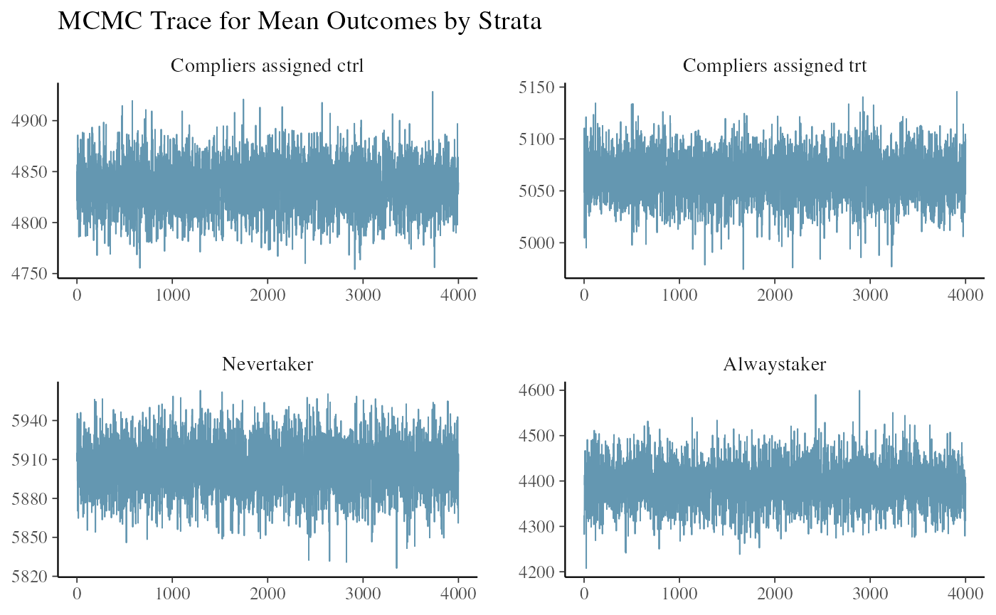
The four plots are the posterior draws of the mean outcomes among the compliers assigned to control, the compliers nudged to treatment, the never-takers, and the always-takers. The poor mixing in the second and the fourth plots warns us about the potential issue of confusing the nudged compliers with the always-takers. We know from this simulation example that the always-takers on average have lower outcomes than the compliers so this explains the dark blue chain underestimating the outcomes among nudged compliers and overestimating the outcomes among always-takers. In this case, the CACE estimate will be underestimated as well.
Before getting the test statistics, we run the weak instrument test to see if the issue of poor mixing is due to a weak instrument.
ivobj$weakIVTest()
#> The instrument is not considered weak, resulting in an estimated 50% of compliers in the population.
No weak instrument issue is detected.
More detailed findings are reported by the same methods. Compared to the results from the above two-side example with good mixing, it overestimates the proportion of never-takers. Both posterior mean and median are underestimated. More uncertainty is reflected in the posterior probability that the CACE is greater than 200. Wider credible intervals are reported.
# Posterior distribution of the strata probability
ivobj$strataProbEstimate()
#> Given the data, we estimate that there is a 50% probability that the unit is a complier, a 38% probability that the unit is a never-taker, and a 13% probability that the unit is an always-taker.
# Posterior probability that CACE is greater than 200
ivobj$calcProb(a = 200)
#> Given the data, we estimate that the probability that the effect is more than 200 is 81%.
# Posterior median of the CACE
ivobj$pointEstimate()
#> [1] 227.0423
# Posterior mean of the CACE
ivobj$pointEstimate(median = FALSE)
#> [1] 227.3359
# 75% credible interval of the CACE
ivobj$credibleInterval()
#> Given the data, we estimate that there is a 75% probability that the CACE is between 191.52 and 263.1.
# 95% credible interval of the CACE
ivobj$credibleInterval(width = 0.95)
#> Given the data, we estimate that there is a 95% probability that the CACE is between 166.17 and 288.01.
In real data analysis, without knowing the actual direction and magnitude of the inaccurate estimation, it is better not to use the posterior mean as the only reported point estimate. The posterior median will be a more robust choice. Posterior probability and credible intervals are faithful characterizations of the uncertainty relevant to decision-making.
The issue of poor mixing can also be identified by the vizdraws method. Users will see bimodal distribution of the posterior for the CACE in the plot.
ivobj$vizdraws(
  display_mode_name = TRUE, breaks = 200,
  break_names = c("< 200", "> 200")
)
Cautionary note 2: weak instrument
Weak instrument refers to an instrument that has a small impact on the treatment. In the noncompliance setting, it means that the assignment barely affects the treatment. In other words, there are many never-takers and always-takers, but a very small proportion of compliers.
A weak instrument, or a small proportion of compliers, could theoretically plague the analysis and the decision-making by
- Posing difficulty in modeling the strata membership due to imbalanced groups sizes, thus the outcomes within each strata, and the CACE.
- Combined with a small sample size, there will be little information contained in the data to update our knowledge about the outcomes among compliers and the CACE, inducing sensitivity to the priors.
- Unreliable point estimate and wider credible intervals of the CACE
- Targeting at a very small proportion of the population where the impact of the treatment is measureable.
We show an example of a weak instrument.
Data simulation
We tweak the proportion of compliers in the data-generating process. We increase the sample size from 200 to 1000 to isolate the issues due to a weak instrument from a small sample size. The issues discovered below shall be further exacerbated with a smaller sample size.
set.seed(1997)
n <- 1000

# Covariates: X observed, U unobserved
X <- rnorm(n)
U <- rbinom(n, 1, 0.5)

## True memberships of principal strata (1:c,2:nt,3:at): S-model depends only on U
true.PS <- rep(0, n)
U1.ind <- (U == 1)
U0.ind <- (U == 0)
num.U1 <- sum(U1.ind)
num.U0 <- sum(U0.ind)
true.PS[U1.ind] <- t(rmultinom(num.U1, 1, c(0.06, 0.7, 0.24))) %*% c(1, 2, 3)
true.PS[U0.ind] <- t(rmultinom(num.U0, 1, c(0.04, 0.7, 0.26))) %*% c(1, 2, 3)

## Treatment assigned: half control & half treatment
Z <- c(rep(0, n / 2), rep(1, n / 2))

## Treatment received: determined by principal strata and treatment assigned
D <- rep(0, n)
c.trt.ind <- (true.PS == 1) & (Z == 1)
c.ctrl.ind <- (true.PS == 1) & (Z == 0)
nt.ind <- (true.PS == 2)
at.ind <- (true.PS == 3)
num.c.trt <- sum(c.trt.ind)
num.c.ctrl <- sum(c.ctrl.ind)
num.nt <- sum(nt.ind)
num.at <- sum(at.ind)
D[at.ind] <- rep(1, num.at)
D[c.trt.ind] <- rep(1, num.c.trt)

## Generate observed outcome: Y-model depend on X, U, D, and principal strata
Y <- rep(0, n)
Y[c.ctrl.ind] <- rnorm(num.c.ctrl,
  mean = 5000 + 100 * X[c.ctrl.ind] - 300 * U[c.ctrl.ind],
  sd = 50
)
Y[c.trt.ind] <- rnorm(num.c.trt,
  mean = 5250 + 100 * X[c.trt.ind] - 300 * U[c.trt.ind],
  sd = 50
)
Y[nt.ind] <- rnorm(num.nt,
  mean = 6000 + 100 * X[nt.ind] - 300 * U[nt.ind],
  sd = 50
)
Y[at.ind] <- rnorm(num.at,
  mean = 4500 + 100 * X[at.ind] - 300 * U[at.ind],
  sd = 50
)


df <- data.frame(Y = Y, Z = Z, D = D, X = X, U = U)
Fitting a BIVA model to the data
The prior specifications stay the same so we skip to the step of fitting a BIVA model to the data.
ivobj <- biva$new(
  data = df, y = "Y", d = "D", z = "Z",
  x_ymodel = c("X"),
  x_smodel = c("X"),
  ER = 1,
  side = 2,
  beta_mean_ymodel = cbind(rep(5000, 4), rep(0, 4)),
  beta_sd_ymodel = cbind(rep(200, 4), rep(200, 4)),
  beta_mean_smodel = matrix(0, 2, 2),
  beta_sd_smodel = matrix(1, 2, 2),
  sigma_shape_ymodel = rep(1, 4),
  sigma_scale_ymodel = rep(1, 4),
  fit = TRUE
)
#>
#> SAMPLING FOR MODEL 'Gaussian' NOW (CHAIN 1).
#> Chain 1:
#> Chain 1: Gradient evaluation took 5e-06 seconds
#> Chain 1: 1000 transitions using 10 leapfrog steps per transition would take 0.05 seconds.
#> Chain 1: Adjust your expectations accordingly!
#> Chain 1:
#> Chain 1:
#> Chain 1: Iteration:    1 / 2000 [  0%]  (Warmup)
#> Chain 1: Iteration:  200 / 2000 [ 10%]  (Warmup)
#> Chain 1: Iteration:  400 / 2000 [ 20%]  (Warmup)
#> Chain 1: Iteration:  600 / 2000 [ 30%]  (Warmup)
#> Chain 1: Iteration:  800 / 2000 [ 40%]  (Warmup)
#> Chain 1: Iteration: 1000 / 2000 [ 50%]  (Warmup)
#> Chain 1: Iteration: 1001 / 2000 [ 50%]  (Sampling)
#> Chain 1: Iteration: 1200 / 2000 [ 60%]  (Sampling)
#> Chain 1: Iteration: 1400 / 2000 [ 70%]  (Sampling)
#> Chain 1: Iteration: 1600 / 2000 [ 80%]  (Sampling)
#> Chain 1: Iteration: 1800 / 2000 [ 90%]  (Sampling)
#> Chain 1: Iteration: 2000 / 2000 [100%]  (Sampling)
#> Chain 1:
#> Chain 1:  Elapsed Time: 0.556 seconds (Warm-up)
#> Chain 1:                0.292 seconds (Sampling)
#> Chain 1:                0.848 seconds (Total)
#> Chain 1:
#>
#> SAMPLING FOR MODEL 'Gaussian' NOW (CHAIN 2).
#> Chain 2:
#> Chain 2: Gradient evaluation took 4e-06 seconds
#> Chain 2: 1000 transitions using 10 leapfrog steps per transition would take 0.04 seconds.
#> Chain 2: Adjust your expectations accordingly!
#> Chain 2:
#> Chain 2:
#> Chain 2: Iteration:    1 / 2000 [  0%]  (Warmup)
#> Chain 2: Iteration:  200 / 2000 [ 10%]  (Warmup)
#> Chain 2: Iteration:  400 / 2000 [ 20%]  (Warmup)
#> Chain 2: Iteration:  600 / 2000 [ 30%]  (Warmup)
#> Chain 2: Iteration:  800 / 2000 [ 40%]  (Warmup)
#> Chain 2: Iteration: 1000 / 2000 [ 50%]  (Warmup)
#> Chain 2: Iteration: 1001 / 2000 [ 50%]  (Sampling)
#> Chain 2: Iteration: 1200 / 2000 [ 60%]  (Sampling)
#> Chain 2: Iteration: 1400 / 2000 [ 70%]  (Sampling)
#> Chain 2: Iteration: 1600 / 2000 [ 80%]  (Sampling)
#> Chain 2: Iteration: 1800 / 2000 [ 90%]  (Sampling)
#> Chain 2: Iteration: 2000 / 2000 [100%]  (Sampling)
#> Chain 2:
#> Chain 2:  Elapsed Time: 0.505 seconds (Warm-up)
#> Chain 2:                0.289 seconds (Sampling)
#> Chain 2:                0.794 seconds (Total)
#> Chain 2:
#>
#> SAMPLING FOR MODEL 'Gaussian' NOW (CHAIN 3).
#> Chain 3:
#> Chain 3: Gradient evaluation took 4e-06 seconds
#> Chain 3: 1000 transitions using 10 leapfrog steps per transition would take 0.04 seconds.
#> Chain 3: Adjust your expectations accordingly!
#> Chain 3:
#> Chain 3:
#> Chain 3: Iteration:    1 / 2000 [  0%]  (Warmup)
#> Chain 3: Iteration:  200 / 2000 [ 10%]  (Warmup)
#> Chain 3: Iteration:  400 / 2000 [ 20%]  (Warmup)
#> Chain 3: Iteration:  600 / 2000 [ 30%]  (Warmup)
#> Chain 3: Iteration:  800 / 2000 [ 40%]  (Warmup)
#> Chain 3: Iteration: 1000 / 2000 [ 50%]  (Warmup)
#> Chain 3: Iteration: 1001 / 2000 [ 50%]  (Sampling)
#> Chain 3: Iteration: 1200 / 2000 [ 60%]  (Sampling)
#> Chain 3: Iteration: 1400 / 2000 [ 70%]  (Sampling)
#> Chain 3: Iteration: 1600 / 2000 [ 80%]  (Sampling)
#> Chain 3: Iteration: 1800 / 2000 [ 90%]  (Sampling)
#> Chain 3: Iteration: 2000 / 2000 [100%]  (Sampling)
#> Chain 3:
#> Chain 3:  Elapsed Time: 0.531 seconds (Warm-up)
#> Chain 3:                0.297 seconds (Sampling)
#> Chain 3:                0.828 seconds (Total)
#> Chain 3:
#>
#> SAMPLING FOR MODEL 'Gaussian' NOW (CHAIN 4).
#> Chain 4:
#> Chain 4: Gradient evaluation took 4e-06 seconds
#> Chain 4: 1000 transitions using 10 leapfrog steps per transition would take 0.04 seconds.
#> Chain 4: Adjust your expectations accordingly!
#> Chain 4:
#> Chain 4:
#> Chain 4: Iteration:    1 / 2000 [  0%]  (Warmup)
#> Chain 4: Iteration:  200 / 2000 [ 10%]  (Warmup)
#> Chain 4: Iteration:  400 / 2000 [ 20%]  (Warmup)
#> Chain 4: Iteration:  600 / 2000 [ 30%]  (Warmup)
#> Chain 4: Iteration:  800 / 2000 [ 40%]  (Warmup)
#> Chain 4: Iteration: 1000 / 2000 [ 50%]  (Warmup)
#> Chain 4: Iteration: 1001 / 2000 [ 50%]  (Sampling)
#> Chain 4: Iteration: 1200 / 2000 [ 60%]  (Sampling)
#> Chain 4: Iteration: 1400 / 2000 [ 70%]  (Sampling)
#> Chain 4: Iteration: 1600 / 2000 [ 80%]  (Sampling)
#> Chain 4: Iteration: 1800 / 2000 [ 90%]  (Sampling)
#> Chain 4: Iteration: 2000 / 2000 [100%]  (Sampling)
#> Chain 4:
#> Chain 4:  Elapsed Time: 0.553 seconds (Warm-up)
#> Chain 4:                0.293 seconds (Sampling)
#> Chain 4:                0.846 seconds (Total)
#> Chain 4:
#> Fitting model to the data
#>
#> SAMPLING FOR MODEL 'Gaussian' NOW (CHAIN 1).
#> Chain 1:
#> Chain 1: Gradient evaluation took 0.001052 seconds
#> Chain 1: 1000 transitions using 10 leapfrog steps per transition would take 10.52 seconds.
#> Chain 1: Adjust your expectations accordingly!
#> Chain 1:
#> Chain 1:
#> Chain 1: Iteration:    1 / 2000 [  0%]  (Warmup)
#> Chain 1: Iteration:  200 / 2000 [ 10%]  (Warmup)
#> Chain 1: Iteration:  400 / 2000 [ 20%]  (Warmup)
#> Chain 1: Iteration:  600 / 2000 [ 30%]  (Warmup)
#> Chain 1: Iteration:  800 / 2000 [ 40%]  (Warmup)
#> Chain 1: Iteration: 1000 / 2000 [ 50%]  (Warmup)
#> Chain 1: Iteration: 1001 / 2000 [ 50%]  (Sampling)
#> Chain 1: Iteration: 1200 / 2000 [ 60%]  (Sampling)
#> Chain 1: Iteration: 1400 / 2000 [ 70%]  (Sampling)
#> Chain 1: Iteration: 1600 / 2000 [ 80%]  (Sampling)
#> Chain 1: Iteration: 1800 / 2000 [ 90%]  (Sampling)
#> Chain 1: Iteration: 2000 / 2000 [100%]  (Sampling)
#> Chain 1:
#> Chain 1:  Elapsed Time: 107.675 seconds (Warm-up)
#> Chain 1:                13.473 seconds (Sampling)
#> Chain 1:                121.148 seconds (Total)
#> Chain 1:
#>
#> SAMPLING FOR MODEL 'Gaussian' NOW (CHAIN 2).
#> Chain 2:
#> Chain 2: Gradient evaluation took 0.000896 seconds
#> Chain 2: 1000 transitions using 10 leapfrog steps per transition would take 8.96 seconds.
#> Chain 2: Adjust your expectations accordingly!
#> Chain 2:
#> Chain 2:
#> Chain 2: Iteration:    1 / 2000 [  0%]  (Warmup)
#> Chain 2: Iteration:  200 / 2000 [ 10%]  (Warmup)
#> Chain 2: Iteration:  400 / 2000 [ 20%]  (Warmup)
#> Chain 2: Iteration:  600 / 2000 [ 30%]  (Warmup)
#> Chain 2: Iteration:  800 / 2000 [ 40%]  (Warmup)
#> Chain 2: Iteration: 1000 / 2000 [ 50%]  (Warmup)
#> Chain 2: Iteration: 1001 / 2000 [ 50%]  (Sampling)
#> Chain 2: Iteration: 1200 / 2000 [ 60%]  (Sampling)
#> Chain 2: Iteration: 1400 / 2000 [ 70%]  (Sampling)
#> Chain 2: Iteration: 1600 / 2000 [ 80%]  (Sampling)
#> Chain 2: Iteration: 1800 / 2000 [ 90%]  (Sampling)
#> Chain 2: Iteration: 2000 / 2000 [100%]  (Sampling)
#> Chain 2:
#> Chain 2:  Elapsed Time: 97.963 seconds (Warm-up)
#> Chain 2:                14.032 seconds (Sampling)
#> Chain 2:                111.995 seconds (Total)
#> Chain 2:
#>
#> SAMPLING FOR MODEL 'Gaussian' NOW (CHAIN 3).
#> Chain 3:
#> Chain 3: Gradient evaluation took 0.000874 seconds
#> Chain 3: 1000 transitions using 10 leapfrog steps per transition would take 8.74 seconds.
#> Chain 3: Adjust your expectations accordingly!
#> Chain 3:
#> Chain 3:
#> Chain 3: Iteration:    1 / 2000 [  0%]  (Warmup)
#> Chain 3: Iteration:  200 / 2000 [ 10%]  (Warmup)
#> Chain 3: Iteration:  400 / 2000 [ 20%]  (Warmup)
#> Chain 3: Iteration:  600 / 2000 [ 30%]  (Warmup)
#> Chain 3: Iteration:  800 / 2000 [ 40%]  (Warmup)
#> Chain 3: Iteration: 1000 / 2000 [ 50%]  (Warmup)
#> Chain 3: Iteration: 1001 / 2000 [ 50%]  (Sampling)
#> Chain 3: Iteration: 1200 / 2000 [ 60%]  (Sampling)
#> Chain 3: Iteration: 1400 / 2000 [ 70%]  (Sampling)
#> Chain 3: Iteration: 1600 / 2000 [ 80%]  (Sampling)
#> Chain 3: Iteration: 1800 / 2000 [ 90%]  (Sampling)
#> Chain 3: Iteration: 2000 / 2000 [100%]  (Sampling)
#> Chain 3:
#> Chain 3:  Elapsed Time: 89.396 seconds (Warm-up)
#> Chain 3:                12.968 seconds (Sampling)
#> Chain 3:                102.364 seconds (Total)
#> Chain 3:
#>
#> SAMPLING FOR MODEL 'Gaussian' NOW (CHAIN 4).
#> Chain 4:
#> Chain 4: Gradient evaluation took 0.000901 seconds
#> Chain 4: 1000 transitions using 10 leapfrog steps per transition would take 9.01 seconds.
#> Chain 4: Adjust your expectations accordingly!
#> Chain 4:
#> Chain 4:
#> Chain 4: Iteration:    1 / 2000 [  0%]  (Warmup)
#> Chain 4: Iteration:  200 / 2000 [ 10%]  (Warmup)
#> Chain 4: Iteration:  400 / 2000 [ 20%]  (Warmup)
#> Chain 4: Iteration:  600 / 2000 [ 30%]  (Warmup)
#> Chain 4: Iteration:  800 / 2000 [ 40%]  (Warmup)
#> Chain 4: Iteration: 1000 / 2000 [ 50%]  (Warmup)
#> Chain 4: Iteration: 1001 / 2000 [ 50%]  (Sampling)
#> Chain 4: Iteration: 1200 / 2000 [ 60%]  (Sampling)
#> Chain 4: Iteration: 1400 / 2000 [ 70%]  (Sampling)
#> Chain 4: Iteration: 1600 / 2000 [ 80%]  (Sampling)
#> Chain 4: Iteration: 1800 / 2000 [ 90%]  (Sampling)
#> Chain 4: Iteration: 2000 / 2000 [100%]  (Sampling)
#> Chain 4:
#> Chain 4:  Elapsed Time: 104.276 seconds (Warm-up)
#> Chain 4:                14.178 seconds (Sampling)
#> Chain 4:                118.454 seconds (Total)
#> Chain 4:
#> Warning: The largest R-hat is 2.41, indicating chains have not mixed.
#> Running the chains for more iterations may help. See
#> https://mc-stan.org/misc/warnings.html#r-hat
#> Warning: Bulk Effective Samples Size (ESS) is too low, indicating posterior means and medians may be unreliable.
#> Running the chains for more iterations may help. See
#> https://mc-stan.org/misc/warnings.html#bulk-ess
#> Warning: Tail Effective Samples Size (ESS) is too low, indicating posterior variances and tail quantiles may be unreliable.
#> Running the chains for more iterations may help. See
#> https://mc-stan.org/misc/warnings.html#tail-ess
#> Warning in initialize(...): Only 50% of the Rhats are less than 1.1Only 50% of
#> n_eff/N are greater than 0.001Only 50% of n_eff are greater than 100
Inspecting the trace plot.
ivobj$tracePlot()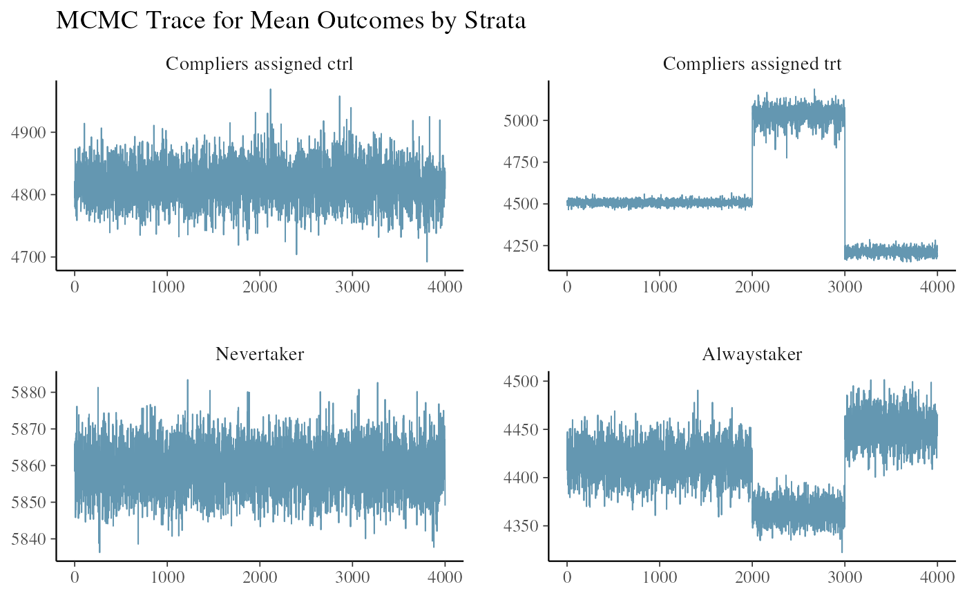
The four plots are the posterior draws of the mean outcomes among the compliers assigned to control, the compliers nudged to treatment, the never-takers, and the always-takers. The poor mixing is detected again.
We run the weak IV test to see if there are any warnings.
ivobj$weakIVTest()
#> The instrument is considered weak, resulting in an estimated 6% of compliers in the population. Posterior point estimates of the CACE might be unreliable.
The weak instrument issue is detected. It warned us about the validity of the estimates if we were to interpret them or apply them to the decision-making.
More detailed findings are reported by the same methods. Compared to the results from the above two-side example with good mixing, it overestimates the proportion of never-takers. Both posterior mean and median are underestimated. More uncertainty is reflected in the posterior probability that the CACE is greater than 200. Wider credible intervals are reported.
# Posterior distribution of the strata probability
ivobj$strataProbEstimate()
#> Given the data, we estimate that there is a 6% probability that the unit is a complier, a 68% probability that the unit is a never-taker, and a 26% probability that the unit is an always-taker.
# Posterior probability that CACE is greater than 200
ivobj$calcProb(a = 200)
#> Given the data, we estimate that the probability that the effect is more than 200 is 16%.
# Posterior median of the CACE
ivobj$pointEstimate()
#> [1] -310.048
# Posterior mean of the CACE
ivobj$pointEstimate(median = FALSE)
#> [1] -250.5781
# 75% credible interval of the CACE
ivobj$credibleInterval()
#> Given the data, we estimate that there is a 75% probability that the CACE is between -601.61 and 222.41.
# 95% credible interval of the CACE
ivobj$credibleInterval(width = 0.95)
#> Given the data, we estimate that there is a 95% probability that the CACE is between -640.02 and 286.69.
The point estimates are way off. Compared with the summary findings from the previous non-weak instrument case, the posterior probability is shrinked and the credible intervals become wider, revealing more uncertainty about the CACE. All these findings indicate that the weak instrument issue is a serious concern, and the results should be interpreted with caution instead of relying too much on the point estimates.
A weak instrument issue can be best avoided by design. Powerful encouragements to events or strong promotions of the features can significantly help with circumventing the issue. Otherwise, it is better to have a larger sample size to avoid the weak instrument issue being further compounded by a small sample size.