Bayesian Instrumental Variable analysis for Binary Outcomes
Yichi Zhang
logit.RmdBelow we demonstrate the overall workflow of the BIVA approach for binary outcomes.
library(biva)Demonstration: two-side noncompliance
Data simulation
We simulate some data from a hypothetical randomized experiment with noncompliance. Those assigned to the treatment group can decide to use the feature or not. Those assigned to the control group may also use the feature since it is available to all. In this case, we have two-side noncompliance where the assigned treated units can opt out and the assigned control can opt in. The outcome metric is a binary variable.
Therefore, there are 3 principal strata: compliers, never-takers, and always-takers.
set.seed(1997)
n <- 200

# Covariates: X observed, U unobserved
X <- rnorm(n)
U <- rbinom(n, 1, 0.5)

## True memberships of principal strata (1:c,2:nt,3:at): S-model depends only on U
true.PS <- rep(0, n)
U1.ind <- (U == 1)
U0.ind <- (U == 0)
num.U1 <- sum(U1.ind)
num.U0 <- sum(U0.ind)
true.PS[U1.ind] <- t(rmultinom(num.U1, 1, c(0.6, 0.3, 0.1))) %*% c(1, 2, 3)
true.PS[U0.ind] <- t(rmultinom(num.U0, 1, c(0.4, 0.5, 0.1))) %*% c(1, 2, 3)

## Treatment assigned: half control & half treatment
Z <- c(rep(0, n / 2), rep(1, n / 2))

## Treatment received: determined by principal strata and treatment assigned
D <- rep(0, n)
c.trt.ind <- (true.PS == 1) & (Z == 1)
c.ctrl.ind <- (true.PS == 1) & (Z == 0)
nt.ind <- (true.PS == 2)
at.ind <- (true.PS == 3)
num.c.trt <- sum(c.trt.ind)
num.c.ctrl <- sum(c.ctrl.ind)
num.nt <- sum(nt.ind)
num.at <- sum(at.ind)
D[at.ind] <- rep(1, num.at)
D[c.trt.ind] <- rep(1, num.c.trt)

## Generate observed outcome: Y-model depend on X, U, D, and principal strata
Y <- rep(0, n)
Y[c.ctrl.ind] <- rbinom(num.c.ctrl, 1, 0.3 + 0.02 * X[c.ctrl.ind] - 0.2 * U[c.ctrl.ind])
Y[c.trt.ind] <- rbinom(num.c.trt, 1, 0.5 + 0.02 * X[c.trt.ind] - 0.2 * U[c.trt.ind])
Y[nt.ind] <- rbinom(num.c.trt, 1, 0.7 + 0.02 * X[nt.ind] - 0.2 * U[nt.ind])
#> Warning in Y[nt.ind] <- rbinom(num.c.trt, 1, 0.7 + 0.02 * X[nt.ind] - 0.2 * :
#> number of items to replace is not a multiple of replacement length
Y[at.ind] <- rbinom(num.c.trt, 1, 0.4 + 0.02 * X[at.ind] - 0.2 * U[at.ind])
#> Warning in Y[at.ind] <- rbinom(num.c.trt, 1, 0.4 + 0.02 * X[at.ind] - 0.2 * :
#> number of items to replace is not a multiple of replacement length

df <- data.frame(Y = Y, Z = Z, D = D, X = X, U = U)
For the strata model, when U = 1, a unit is a complier, a never-taker, or an always-taker with probability 0.6, 0.3, and 0.1, respectively. When U = 0, a unit is a complier, a never-taker, or an always-taker with probability 0.4, 0.5, and 0.1, respectively.
The outcome models are by different strata-nudge combinations. The compliers may adopt the treatment or not depending on the assigned nudge, and thus have two outcome models by treatment groups. The never-takers will never adopt the treatment feature. The always-takers will always adopt the treatment feature. We assume away the direct effect of the nudge here so there is only one outcome model for never-takers, and also one model for always-takers.
The four outcome models depend on both the observed X and the unobserved U with the same slopes. The contrast between the intercepts of the outcome models for compliers then becomes the CACE of the feature, which is 0.5 - 0.3 = 20%.
OLS analysis
We again fit an OLS model with the adopted treatment D and the observed covariate X to see the caveats.
OLS <- lm(data = df, formula = Y ~ D + X)
summary(OLS)
#>
#> Call:
#> lm(formula = Y ~ D + X, data = df)
#>
#> Residuals:
#>     Min      1Q  Median      3Q     Max
#> -0.3833 -0.3666 -0.3602  0.6324  0.6513
#>
#> Coefficients:
#>              Estimate Std. Error t value Pr(>|t|)
#> (Intercept)  0.366418   0.043140   8.494 4.85e-15 ***
#> D           -0.005740   0.071484  -0.080    0.936
#> X           -0.005527   0.034460  -0.160    0.873
#> ---
#> Signif. codes:  0 '***' 0.001 '**' 0.01 '*' 0.05 '.' 0.1 ' ' 1
#>
#> Residual standard error: 0.485 on 197 degrees of freedom
#> Multiple R-squared:  0.0001673,  Adjusted R-squared:  -0.009983
#> F-statistic: 0.01648 on 2 and 197 DF,  p-value: 0.9837
confint(OLS, "D")
#>        2.5 %    97.5 %
#> D -0.1467124 0.1352323
It returns an uninformative insignificant negative estimate of the treatment effect.
We restart the BIVA workflow to get more insight into the impact.
Prior predictive checking
The outcome type is specified by having y_type = “binary”. We assume exclusion restriction, so ER = 1. With two-side noncompliance, we set side = 2. The parameters in the prior distributions are specified as well. We first look into what the prior distributions assume about the parameters.
ivobj <- biva$new(
  data = df, y = "Y", d = "D", z = "Z",
  x_ymodel = c("X"),
  x_smodel = c("X"),
  y_type = "binary",
  ER = 1,
  side = 2,
  beta_mean_ymodel = matrix(0, 4, 2),
  beta_sd_ymodel = matrix(1, 4, 2),
  beta_mean_smodel = matrix(0, 2, 2),
  beta_sd_smodel = matrix(1, 2, 2),
  fit = FALSE
)
#>
#> SAMPLING FOR MODEL 'logit' NOW (CHAIN 1).
#> Chain 1:
#> Chain 1: Gradient evaluation took 5e-06 seconds
#> Chain 1: 1000 transitions using 10 leapfrog steps per transition would take 0.05 seconds.
#> Chain 1: Adjust your expectations accordingly!
#> Chain 1:
#> Chain 1:
#> Chain 1: Iteration:    1 / 2000 [  0%]  (Warmup)
#> Chain 1: Iteration:  200 / 2000 [ 10%]  (Warmup)
#> Chain 1: Iteration:  400 / 2000 [ 20%]  (Warmup)
#> Chain 1: Iteration:  600 / 2000 [ 30%]  (Warmup)
#> Chain 1: Iteration:  800 / 2000 [ 40%]  (Warmup)
#> Chain 1: Iteration: 1000 / 2000 [ 50%]  (Warmup)
#> Chain 1: Iteration: 1001 / 2000 [ 50%]  (Sampling)
#> Chain 1: Iteration: 1200 / 2000 [ 60%]  (Sampling)
#> Chain 1: Iteration: 1400 / 2000 [ 70%]  (Sampling)
#> Chain 1: Iteration: 1600 / 2000 [ 80%]  (Sampling)
#> Chain 1: Iteration: 1800 / 2000 [ 90%]  (Sampling)
#> Chain 1: Iteration: 2000 / 2000 [100%]  (Sampling)
#> Chain 1:
#> Chain 1:  Elapsed Time: 0.081 seconds (Warm-up)
#> Chain 1:                0.082 seconds (Sampling)
#> Chain 1:                0.163 seconds (Total)
#> Chain 1:
#>
#> SAMPLING FOR MODEL 'logit' NOW (CHAIN 2).
#> Chain 2:
#> Chain 2: Gradient evaluation took 3e-06 seconds
#> Chain 2: 1000 transitions using 10 leapfrog steps per transition would take 0.03 seconds.
#> Chain 2: Adjust your expectations accordingly!
#> Chain 2:
#> Chain 2:
#> Chain 2: Iteration:    1 / 2000 [  0%]  (Warmup)
#> Chain 2: Iteration:  200 / 2000 [ 10%]  (Warmup)
#> Chain 2: Iteration:  400 / 2000 [ 20%]  (Warmup)
#> Chain 2: Iteration:  600 / 2000 [ 30%]  (Warmup)
#> Chain 2: Iteration:  800 / 2000 [ 40%]  (Warmup)
#> Chain 2: Iteration: 1000 / 2000 [ 50%]  (Warmup)
#> Chain 2: Iteration: 1001 / 2000 [ 50%]  (Sampling)
#> Chain 2: Iteration: 1200 / 2000 [ 60%]  (Sampling)
#> Chain 2: Iteration: 1400 / 2000 [ 70%]  (Sampling)
#> Chain 2: Iteration: 1600 / 2000 [ 80%]  (Sampling)
#> Chain 2: Iteration: 1800 / 2000 [ 90%]  (Sampling)
#> Chain 2: Iteration: 2000 / 2000 [100%]  (Sampling)
#> Chain 2:
#> Chain 2:  Elapsed Time: 0.08 seconds (Warm-up)
#> Chain 2:                0.082 seconds (Sampling)
#> Chain 2:                0.162 seconds (Total)
#> Chain 2:
#>
#> SAMPLING FOR MODEL 'logit' NOW (CHAIN 3).
#> Chain 3:
#> Chain 3: Gradient evaluation took 3e-06 seconds
#> Chain 3: 1000 transitions using 10 leapfrog steps per transition would take 0.03 seconds.
#> Chain 3: Adjust your expectations accordingly!
#> Chain 3:
#> Chain 3:
#> Chain 3: Iteration:    1 / 2000 [  0%]  (Warmup)
#> Chain 3: Iteration:  200 / 2000 [ 10%]  (Warmup)
#> Chain 3: Iteration:  400 / 2000 [ 20%]  (Warmup)
#> Chain 3: Iteration:  600 / 2000 [ 30%]  (Warmup)
#> Chain 3: Iteration:  800 / 2000 [ 40%]  (Warmup)
#> Chain 3: Iteration: 1000 / 2000 [ 50%]  (Warmup)
#> Chain 3: Iteration: 1001 / 2000 [ 50%]  (Sampling)
#> Chain 3: Iteration: 1200 / 2000 [ 60%]  (Sampling)
#> Chain 3: Iteration: 1400 / 2000 [ 70%]  (Sampling)
#> Chain 3: Iteration: 1600 / 2000 [ 80%]  (Sampling)
#> Chain 3: Iteration: 1800 / 2000 [ 90%]  (Sampling)
#> Chain 3: Iteration: 2000 / 2000 [100%]  (Sampling)
#> Chain 3:
#> Chain 3:  Elapsed Time: 0.081 seconds (Warm-up)
#> Chain 3:                0.082 seconds (Sampling)
#> Chain 3:                0.163 seconds (Total)
#> Chain 3:
#>
#> SAMPLING FOR MODEL 'logit' NOW (CHAIN 4).
#> Chain 4:
#> Chain 4: Gradient evaluation took 3e-06 seconds
#> Chain 4: 1000 transitions using 10 leapfrog steps per transition would take 0.03 seconds.
#> Chain 4: Adjust your expectations accordingly!
#> Chain 4:
#> Chain 4:
#> Chain 4: Iteration:    1 / 2000 [  0%]  (Warmup)
#> Chain 4: Iteration:  200 / 2000 [ 10%]  (Warmup)
#> Chain 4: Iteration:  400 / 2000 [ 20%]  (Warmup)
#> Chain 4: Iteration:  600 / 2000 [ 30%]  (Warmup)
#> Chain 4: Iteration:  800 / 2000 [ 40%]  (Warmup)
#> Chain 4: Iteration: 1000 / 2000 [ 50%]  (Warmup)
#> Chain 4: Iteration: 1001 / 2000 [ 50%]  (Sampling)
#> Chain 4: Iteration: 1200 / 2000 [ 60%]  (Sampling)
#> Chain 4: Iteration: 1400 / 2000 [ 70%]  (Sampling)
#> Chain 4: Iteration: 1600 / 2000 [ 80%]  (Sampling)
#> Chain 4: Iteration: 1800 / 2000 [ 90%]  (Sampling)
#> Chain 4: Iteration: 2000 / 2000 [100%]  (Sampling)
#> Chain 4:
#> Chain 4:  Elapsed Time: 0.08 seconds (Warm-up)
#> Chain 4:                0.08 seconds (Sampling)
#> Chain 4:                0.16 seconds (Total)
#> Chain 4:

ivobj$plotPrior()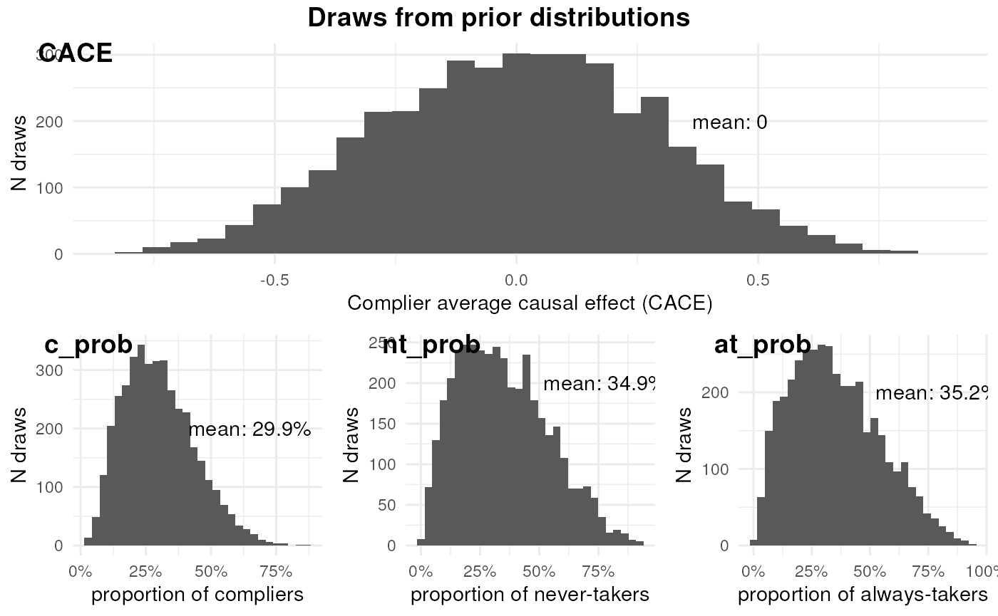
By prior, the effect of the AI-powered dubbing feature among compliers is negligible. The proportions of compliers, never-takers, and always-takers are similar.
Fitting a BIVA model to the data
Now we fit a BIVA model to the data.
ivobj <- biva$new(
  data = df, y = "Y", d = "D", z = "Z",
  x_ymodel = c("X"),
  x_smodel = c("X"),
  y_type = "binary",
  ER = 1,
  side = 2,
  beta_mean_ymodel = matrix(0, 4, 2),
  beta_sd_ymodel = matrix(1, 4, 2),
  beta_mean_smodel = matrix(0, 2, 2),
  beta_sd_smodel = matrix(1, 2, 2),
  fit = TRUE
)
#>
#> SAMPLING FOR MODEL 'logit' NOW (CHAIN 1).
#> Chain 1:
#> Chain 1: Gradient evaluation took 5e-06 seconds
#> Chain 1: 1000 transitions using 10 leapfrog steps per transition would take 0.05 seconds.
#> Chain 1: Adjust your expectations accordingly!
#> Chain 1:
#> Chain 1:
#> Chain 1: Iteration:    1 / 2000 [  0%]  (Warmup)
#> Chain 1: Iteration:  200 / 2000 [ 10%]  (Warmup)
#> Chain 1: Iteration:  400 / 2000 [ 20%]  (Warmup)
#> Chain 1: Iteration:  600 / 2000 [ 30%]  (Warmup)
#> Chain 1: Iteration:  800 / 2000 [ 40%]  (Warmup)
#> Chain 1: Iteration: 1000 / 2000 [ 50%]  (Warmup)
#> Chain 1: Iteration: 1001 / 2000 [ 50%]  (Sampling)
#> Chain 1: Iteration: 1200 / 2000 [ 60%]  (Sampling)
#> Chain 1: Iteration: 1400 / 2000 [ 70%]  (Sampling)
#> Chain 1: Iteration: 1600 / 2000 [ 80%]  (Sampling)
#> Chain 1: Iteration: 1800 / 2000 [ 90%]  (Sampling)
#> Chain 1: Iteration: 2000 / 2000 [100%]  (Sampling)
#> Chain 1:
#> Chain 1:  Elapsed Time: 0.083 seconds (Warm-up)
#> Chain 1:                0.085 seconds (Sampling)
#> Chain 1:                0.168 seconds (Total)
#> Chain 1:
#>
#> SAMPLING FOR MODEL 'logit' NOW (CHAIN 2).
#> Chain 2:
#> Chain 2: Gradient evaluation took 3e-06 seconds
#> Chain 2: 1000 transitions using 10 leapfrog steps per transition would take 0.03 seconds.
#> Chain 2: Adjust your expectations accordingly!
#> Chain 2:
#> Chain 2:
#> Chain 2: Iteration:    1 / 2000 [  0%]  (Warmup)
#> Chain 2: Iteration:  200 / 2000 [ 10%]  (Warmup)
#> Chain 2: Iteration:  400 / 2000 [ 20%]  (Warmup)
#> Chain 2: Iteration:  600 / 2000 [ 30%]  (Warmup)
#> Chain 2: Iteration:  800 / 2000 [ 40%]  (Warmup)
#> Chain 2: Iteration: 1000 / 2000 [ 50%]  (Warmup)
#> Chain 2: Iteration: 1001 / 2000 [ 50%]  (Sampling)
#> Chain 2: Iteration: 1200 / 2000 [ 60%]  (Sampling)
#> Chain 2: Iteration: 1400 / 2000 [ 70%]  (Sampling)
#> Chain 2: Iteration: 1600 / 2000 [ 80%]  (Sampling)
#> Chain 2: Iteration: 1800 / 2000 [ 90%]  (Sampling)
#> Chain 2: Iteration: 2000 / 2000 [100%]  (Sampling)
#> Chain 2:
#> Chain 2:  Elapsed Time: 0.084 seconds (Warm-up)
#> Chain 2:                0.083 seconds (Sampling)
#> Chain 2:                0.167 seconds (Total)
#> Chain 2:
#>
#> SAMPLING FOR MODEL 'logit' NOW (CHAIN 3).
#> Chain 3:
#> Chain 3: Gradient evaluation took 3e-06 seconds
#> Chain 3: 1000 transitions using 10 leapfrog steps per transition would take 0.03 seconds.
#> Chain 3: Adjust your expectations accordingly!
#> Chain 3:
#> Chain 3:
#> Chain 3: Iteration:    1 / 2000 [  0%]  (Warmup)
#> Chain 3: Iteration:  200 / 2000 [ 10%]  (Warmup)
#> Chain 3: Iteration:  400 / 2000 [ 20%]  (Warmup)
#> Chain 3: Iteration:  600 / 2000 [ 30%]  (Warmup)
#> Chain 3: Iteration:  800 / 2000 [ 40%]  (Warmup)
#> Chain 3: Iteration: 1000 / 2000 [ 50%]  (Warmup)
#> Chain 3: Iteration: 1001 / 2000 [ 50%]  (Sampling)
#> Chain 3: Iteration: 1200 / 2000 [ 60%]  (Sampling)
#> Chain 3: Iteration: 1400 / 2000 [ 70%]  (Sampling)
#> Chain 3: Iteration: 1600 / 2000 [ 80%]  (Sampling)
#> Chain 3: Iteration: 1800 / 2000 [ 90%]  (Sampling)
#> Chain 3: Iteration: 2000 / 2000 [100%]  (Sampling)
#> Chain 3:
#> Chain 3:  Elapsed Time: 0.081 seconds (Warm-up)
#> Chain 3:                0.084 seconds (Sampling)
#> Chain 3:                0.165 seconds (Total)
#> Chain 3:
#>
#> SAMPLING FOR MODEL 'logit' NOW (CHAIN 4).
#> Chain 4:
#> Chain 4: Gradient evaluation took 3e-06 seconds
#> Chain 4: 1000 transitions using 10 leapfrog steps per transition would take 0.03 seconds.
#> Chain 4: Adjust your expectations accordingly!
#> Chain 4:
#> Chain 4:
#> Chain 4: Iteration:    1 / 2000 [  0%]  (Warmup)
#> Chain 4: Iteration:  200 / 2000 [ 10%]  (Warmup)
#> Chain 4: Iteration:  400 / 2000 [ 20%]  (Warmup)
#> Chain 4: Iteration:  600 / 2000 [ 30%]  (Warmup)
#> Chain 4: Iteration:  800 / 2000 [ 40%]  (Warmup)
#> Chain 4: Iteration: 1000 / 2000 [ 50%]  (Warmup)
#> Chain 4: Iteration: 1001 / 2000 [ 50%]  (Sampling)
#> Chain 4: Iteration: 1200 / 2000 [ 60%]  (Sampling)
#> Chain 4: Iteration: 1400 / 2000 [ 70%]  (Sampling)
#> Chain 4: Iteration: 1600 / 2000 [ 80%]  (Sampling)
#> Chain 4: Iteration: 1800 / 2000 [ 90%]  (Sampling)
#> Chain 4: Iteration: 2000 / 2000 [100%]  (Sampling)
#> Chain 4:
#> Chain 4:  Elapsed Time: 0.082 seconds (Warm-up)
#> Chain 4:                0.082 seconds (Sampling)
#> Chain 4:                0.164 seconds (Total)
#> Chain 4:
#> Fitting model to the data
#>
#> SAMPLING FOR MODEL 'logit' NOW (CHAIN 1).
#> Chain 1:
#> Chain 1: Gradient evaluation took 0.000207 seconds
#> Chain 1: 1000 transitions using 10 leapfrog steps per transition would take 2.07 seconds.
#> Chain 1: Adjust your expectations accordingly!
#> Chain 1:
#> Chain 1:
#> Chain 1: Iteration:    1 / 2000 [  0%]  (Warmup)
#> Chain 1: Iteration:  200 / 2000 [ 10%]  (Warmup)
#> Chain 1: Iteration:  400 / 2000 [ 20%]  (Warmup)
#> Chain 1: Iteration:  600 / 2000 [ 30%]  (Warmup)
#> Chain 1: Iteration:  800 / 2000 [ 40%]  (Warmup)
#> Chain 1: Iteration: 1000 / 2000 [ 50%]  (Warmup)
#> Chain 1: Iteration: 1001 / 2000 [ 50%]  (Sampling)
#> Chain 1: Iteration: 1200 / 2000 [ 60%]  (Sampling)
#> Chain 1: Iteration: 1400 / 2000 [ 70%]  (Sampling)
#> Chain 1: Iteration: 1600 / 2000 [ 80%]  (Sampling)
#> Chain 1: Iteration: 1800 / 2000 [ 90%]  (Sampling)
#> Chain 1: Iteration: 2000 / 2000 [100%]  (Sampling)
#> Chain 1:
#> Chain 1:  Elapsed Time: 2.065 seconds (Warm-up)
#> Chain 1:                1.718 seconds (Sampling)
#> Chain 1:                3.783 seconds (Total)
#> Chain 1:
#>
#> SAMPLING FOR MODEL 'logit' NOW (CHAIN 2).
#> Chain 2:
#> Chain 2: Gradient evaluation took 0.00019 seconds
#> Chain 2: 1000 transitions using 10 leapfrog steps per transition would take 1.9 seconds.
#> Chain 2: Adjust your expectations accordingly!
#> Chain 2:
#> Chain 2:
#> Chain 2: Iteration:    1 / 2000 [  0%]  (Warmup)
#> Chain 2: Iteration:  200 / 2000 [ 10%]  (Warmup)
#> Chain 2: Iteration:  400 / 2000 [ 20%]  (Warmup)
#> Chain 2: Iteration:  600 / 2000 [ 30%]  (Warmup)
#> Chain 2: Iteration:  800 / 2000 [ 40%]  (Warmup)
#> Chain 2: Iteration: 1000 / 2000 [ 50%]  (Warmup)
#> Chain 2: Iteration: 1001 / 2000 [ 50%]  (Sampling)
#> Chain 2: Iteration: 1200 / 2000 [ 60%]  (Sampling)
#> Chain 2: Iteration: 1400 / 2000 [ 70%]  (Sampling)
#> Chain 2: Iteration: 1600 / 2000 [ 80%]  (Sampling)
#> Chain 2: Iteration: 1800 / 2000 [ 90%]  (Sampling)
#> Chain 2: Iteration: 2000 / 2000 [100%]  (Sampling)
#> Chain 2:
#> Chain 2:  Elapsed Time: 1.955 seconds (Warm-up)
#> Chain 2:                1.741 seconds (Sampling)
#> Chain 2:                3.696 seconds (Total)
#> Chain 2:
#>
#> SAMPLING FOR MODEL 'logit' NOW (CHAIN 3).
#> Chain 3:
#> Chain 3: Gradient evaluation took 0.00019 seconds
#> Chain 3: 1000 transitions using 10 leapfrog steps per transition would take 1.9 seconds.
#> Chain 3: Adjust your expectations accordingly!
#> Chain 3:
#> Chain 3:
#> Chain 3: Iteration:    1 / 2000 [  0%]  (Warmup)
#> Chain 3: Iteration:  200 / 2000 [ 10%]  (Warmup)
#> Chain 3: Iteration:  400 / 2000 [ 20%]  (Warmup)
#> Chain 3: Iteration:  600 / 2000 [ 30%]  (Warmup)
#> Chain 3: Iteration:  800 / 2000 [ 40%]  (Warmup)
#> Chain 3: Iteration: 1000 / 2000 [ 50%]  (Warmup)
#> Chain 3: Iteration: 1001 / 2000 [ 50%]  (Sampling)
#> Chain 3: Iteration: 1200 / 2000 [ 60%]  (Sampling)
#> Chain 3: Iteration: 1400 / 2000 [ 70%]  (Sampling)
#> Chain 3: Iteration: 1600 / 2000 [ 80%]  (Sampling)
#> Chain 3: Iteration: 1800 / 2000 [ 90%]  (Sampling)
#> Chain 3: Iteration: 2000 / 2000 [100%]  (Sampling)
#> Chain 3:
#> Chain 3:  Elapsed Time: 1.94 seconds (Warm-up)
#> Chain 3:                1.747 seconds (Sampling)
#> Chain 3:                3.687 seconds (Total)
#> Chain 3:
#>
#> SAMPLING FOR MODEL 'logit' NOW (CHAIN 4).
#> Chain 4:
#> Chain 4: Gradient evaluation took 0.000196 seconds
#> Chain 4: 1000 transitions using 10 leapfrog steps per transition would take 1.96 seconds.
#> Chain 4: Adjust your expectations accordingly!
#> Chain 4:
#> Chain 4:
#> Chain 4: Iteration:    1 / 2000 [  0%]  (Warmup)
#> Chain 4: Iteration:  200 / 2000 [ 10%]  (Warmup)
#> Chain 4: Iteration:  400 / 2000 [ 20%]  (Warmup)
#> Chain 4: Iteration:  600 / 2000 [ 30%]  (Warmup)
#> Chain 4: Iteration:  800 / 2000 [ 40%]  (Warmup)
#> Chain 4: Iteration: 1000 / 2000 [ 50%]  (Warmup)
#> Chain 4: Iteration: 1001 / 2000 [ 50%]  (Sampling)
#> Chain 4: Iteration: 1200 / 2000 [ 60%]  (Sampling)
#> Chain 4: Iteration: 1400 / 2000 [ 70%]  (Sampling)
#> Chain 4: Iteration: 1600 / 2000 [ 80%]  (Sampling)
#> Chain 4: Iteration: 1800 / 2000 [ 90%]  (Sampling)
#> Chain 4: Iteration: 2000 / 2000 [100%]  (Sampling)
#> Chain 4:
#> Chain 4:  Elapsed Time: 1.898 seconds (Warm-up)
#> Chain 4:                1.67 seconds (Sampling)
#> Chain 4:                3.568 seconds (Total)
#> Chain 4:
#> Found more than one class "Rcpp_rstantools_model_logit" in cache; using the first, from namespace 'biva'
#> Also defined by 'im'
#> Found more than one class "Rcpp_rstantools_model_logit" in cache; using the first, from namespace 'biva'
#> Also defined by 'im'
#> All diagnostics look fine
We look at the trace plot of outcomes in each strata. The four plots are the posterior draws of the mean outcomes among the compliers assinged to control, the compliers nudged to treatment, the never-takers, and the always-takers.
ivobj$tracePlot()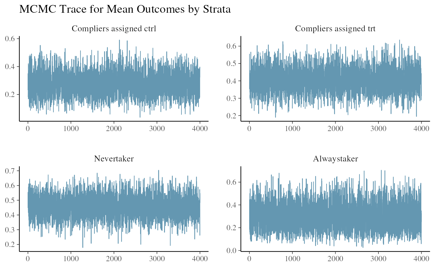
The convergence and mixing look good.
We run the weak instrument test.
ivobj$weakIVTest()
#> The instrument is not considered weak, resulting in an estimated 54% of compliers in the population.
No weak instrument issue is detected.
We can use the following methods to summarize our findings:
# Posterior distribution of the strata probability
ivobj$strataProbEstimate()
#> Given the data, we estimate that there is a 54% probability that the unit is a complier, a 36% probability that the unit is a never-taker, and a 9% probability that the unit is an always-taker.
# Posterior probability that CACE is greater than 0.1
ivobj$calcProb(a = 0.1)
#> Given the data, we estimate that the probability that the effect is more than 0.1 is 61%.
# Posterior median of the CACE
ivobj$pointEstimate()
#> [1] 0.1315855
# Posterior mean of the CACE
ivobj$pointEstimate(median = FALSE)
#> [1] 0.1295604
# 75% credible interval of the CACE
ivobj$credibleInterval()
#> Given the data, we estimate that there is a 75% probability that the CACE is between 0 and 0.26.
# 95% credible interval of the CACE
ivobj$credibleInterval(width = 0.95)
#> Given the data, we estimate that there is a 95% probability that the CACE is between -0.08 and 0.34.
The posterior returns informative conclusions on the impact of the treatment.
Visualizations of how the data updates our knowledge about the impact by comparing its posterior distribution with the prior can be done by running the following methods. We hide them here.
ivobj$vizdraws(
  display_mode_name = TRUE, breaks = 0.1,
  break_names = c("< 0.1", "> 0.1")
)
ivobj$lollipop(threshold = 0.1, mediumText = 8)