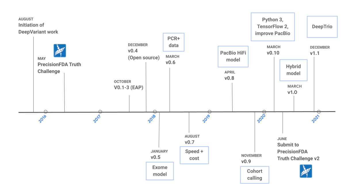
DeepVariant over the years
Authors:


 Alexey Kolesnikov
 Howard Yang

Introduction
The development of DeepVariant was motivated by the following question: if computational biologists can examine pileup images to establish the validity of variants, can an image classification model perform the same task? To answer this question, we began working on DeepVariant in 2015, and the first open-source version (v0.4) of the software was released in late 2017. Since v0.4, the project has come a long way, and there have been eight additional releases, as shown in Figure 1. We originally began development on Illumina whole-genome sequencing (WSG) data, and the first release included one model for this data type. Over the years, we have added support for additional sequencing technologies, and we now provide models for Illumina whole-exome sequencing (WES) data, Pacific Bioscience (PacBio) HiFi data, and a hybrid model for Illumina and PacBio WGS data combined. We have also collaborated with a team at UC Santa Cruz to train DeepVariant using Oxford Nanopore data. The resulting tool, PEPPER-DeepVariant, uses PEPPER to generate candidates more effectively for Nanopore data. In addition to new models, new capabilities have been added, such as the best practices for cohort calling in v0.9 and DeepTrio, a trio and duo caller, in v1.1. For each release, we focus on building highly-accurate models, reducing runtime, and improving the user experience. In this post, we summarize the improvements in accuracy and runtime over the years and highlight a few categories of changes that have led to these improvements.
Accuracy
To balance both precision and recall, we benchmark F1 for each model type and document the results through our case studies. Since these case studies look at just one sample, we also internally assess performance on additional samples to ensure that our models generalize well. Improvements in F1 have been driven by a few different areas: additional input information, expanded training datasets, and higher quality labels. Figure 2 shows error counts over time for the WGS and PacBio models. We visualize error counts rather than F1, since changes in F1 are small, but this still corresponds to significant differences in error counts. We evaluated each version of DeepVariant on HG003 using the latest version of the truth sets, v4.2.1. Chromosome 20 is never used for training, so Figure 2 only shows numbers for that region. We do not include WES numbers in this figure as the full set of chromosomes was not left out of training for all versions, and restricting to chromosome 20 results in very few variants. Additionally, we have only released one version of the Hybrid model, so that is also not included in this historical analysis.


The training samples and truth sets used for training each version vary, so looking at multiple datasets provides a more complete picture of progress. To facilitate more extended benchmarking, we recently released a benchmark set to the community containing 36 WGS runs and 54 WES samples with varying properties (e.g. multiple genomes, sequencers, sample preparation methods, and capture technologies) along with a manuscript. We hope that this dataset is useful to the community for developing methods that perform well across a variety of datasets.
Additional Input Information
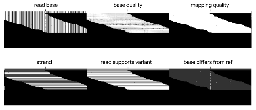
The latest DeepVariant models all use the six channels of information shown in Figure 3: bases, base qualities, mapping qualities, strand information, whether reads support the candidate variant, and whether bases differ from the reference sequence. Mapping quality, strand, and whether the read supports the candidate variant are read-level features, whereas the other features differ for each base. Some models, such as the PacBio model, can include additional channels as well. Each set of features is encoded in a separate channel, and channels are stacked to form a three-dimensional pileup image of bases and associated information.
Over time, these pileup images have changed as we have removed older channels and added new ones. In addition to the six channels, the production PacBio model can now include up to three additional channels: two channels for alt-aligned pileups, in which reads are aligned not just to the reference genome but also to alternate alleles, and a channel representing the haplotype for each read. The result of these additional features is better indel performance on PacBio data. Alt-aligned pileups reduced indel errors by 24%, and the haplotype channel resulted in a 22% error reduction.
Training Data
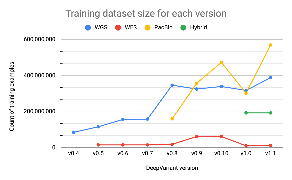
Our training datasets consist of samples from multiple genomes, sequencers, and preparation methods (PCR-free vs. PCR positive) and range from around 13 million to 570 million examples, depending on the model type. Each example corresponds to a putative variant. Using a dataset that is large enough and includes a variety of properties is important for training models that can generalize to real-world data. The size of our training datasets for Illumina WGS and PacBio models have increased as we have added additional BAM files and implemented data augmentations techniques. The hybrid model dataset has not changed since its initial release.
The Illumina WES dataset is much smaller than other datasets, as shown in Figure 4, for a number of reasons. For each BAM file in the dataset, we generate many fewer examples since we consider only the exome regions. The parameters of the Illumina WES model are also initialized from the Illumina WGS model rather than an ImageNet checkpoint. This allows us to leverage learnings from WGS data, for which we have many training examples, and reduces the need for WES data, which is more limited. This training strategy has also been used by external groups, such as Regeneron, who have trained custom DeepVariant models for their use cases. With v1.0, we reduced the size of this dataset compared to previous versions in order to include a more varied set of samples. Prior to v1.0, our WES samples were primarily from HG001, but we have now added additional samples (HG002-7) and reduced the number of HG001 samples.
Performance improvements in machine learning generally come from better data or better models. For DeepVariant, data-centric improvements have been fruitful. Lower performance on specific data types have been addressed by adding representative samples to the training dataset. In v0.6 and v0.8, we improved accuracy of the Illumina WGS model on PCR+ and NovaSeq data, respectively, by including additional samples from those data types during training.
Besides adding more samples, we have also used data augmentation strategies to further expand our datasets. For each BAM file, we downsample reads at multiple fractions to simulate lower coverage data. In addition to creating more training examples, this approach also allows DeepVariant models to generalize across coverages at inference time.
Changes to the core algorithm have also contributed to changes in the training data composition. Candidate variants for training and inference are generated through a very sensitive approach that considers the level of support for a given variant. If the proportion of reads supporting a candidate variant is higher than a minimum threshold, a candidate is generated. In earlier versions of DeepVariant, this threshold was the same across models and variant types. We’ve improved this approach by adding more granularity. For example, a higher threshold is used for PacBio indels than Illumina indels. Indel errors are the dominant error mode in PacBio data, so a lower value results in a very high number of negative examples.
Labels
The techniques mentioned above allow us to generate additional examples, but they do not affect the labels assigned to these examples. Our labels are generated using the truth sets produced by NIST Genome in a Bottle Consortium (GIAB). Creating labels from the truth sets is not always straightforward as we must consider representational differences that may exist between candidate variants and the truth VCF. GIAB regularly improves these truth sets and expands the regions that are confidently benchmarked. For example, the latest versions of the truth sets were built using GRCh38, eliminating the need to lift over coordinates from GRCh37, which can be error-prone, and better capturing regions with segmental duplications.
Runtime

Running inference with DeepVariant consists of three steps: make_examples identifies candidates and generates TensorFlow examples (tf.Examples) for each candidate. These tf.Examples are passed through a pretrained neural network for the appropriate data type during the call_variants step. This step writes out predictions and relevant metadata as well. The postprocess_variants step turns the predictions into a final genotype and writes out a VCF with additional metadata.
Leveraging tools developed by other groups has allowed us to greatly reduce DeepVariant runtimes. In v0.7, we switched to a version of TensorFlow developed by Intel that is optimized for the AVX-512 instruction set. This dramatically reduced the runtime of the call_variants step on CPU by about 75%, as shown in Figure 5. More recently, we have worked with another group at Intel to add an option for running DeepVariant with the OpenVINO toolkit, which can reduce runtime by about 25%.
Conclusion
The answer to our original question is clear: deep neural networks can learn to call variants in pileup images with high accuracy and capture signals that are difficult for humans to identify. If you have not already tried playing against DeepVariant, we encourage you to take a look at this Colab notebook. Despite overall high accuracy, variant calling remains challenging, especially in certain regions such as the MHC. We hope to continue innovating on this problem in future releases, while also ensuring that our tools are efficient and user-friendly.