Variational inference for polygenic risk scores
Authors:

On the Genomics team in Google Health AI, we think a lot about polygenic risk scores (PRS). One concept we have been interested in is black box variational inference (bbVI) for crafting better PRS. Black box variational inference is a form of variational inference (VI) that solves the optimization problem using stochastic optimization and automatic differentiation. This is a cool technique because it allows the practitioner a high degree of flexibility on the statistical modeling side as compared to methods such as Markov-chain Monte Carlo (MCMC). If you agree, or even if you are only vaguely familiar with some words in this paragraph but think they sound enticing, please keep reading!
Given our interest in VI, we were excited to see a preprint from Zabad et al. posted in May of 2022 that introduces the key concepts for using VI to create PRS. They provide great baseline results using a traditional VI approach. However, traditional VI does not employ the black box technique which translates into less modeling flexibility. We believe that bbVI implemented using libraries such as TensorFlow Probability has a lot of potential to be a powerful and flexible methodology for building Bayesian methods, so we figured a blog post laying out some of the basics might be useful for the community.
Here, we first give background context on PRS, LDpred, MCMC and variational inference. If you are already familiar with these concepts, please feel free to skip those sections and head right to the “bbVI + PRS = bbviPRS” section, where we introduce bbviPRS: a method to construct a PRS from GWAS summary statistics that uses black box variational inference. We also provide a companion colab with an implementation of the method.
Polygenic risk scores (PRS) and LDpred
Over the last decade, PRS have become the canonical way to think about how many genetic variants express their influence over complex human traits. As a result, there has been a lot of effort focused on making bigger and more accurate PRS. The key idea behind a PRS is quite simple: sum the effects of each of many genetic variants to create a score that is predictive of the trait or disease.
One of the most well known and widely used methods for developing PRS is called LDpred (and more recently LDpred2). LDPred introduced a really clever idea to infer the true effects of each genetic variant by using summary statistics taken from a standard GWAS, and modifying the variant effects to account for the correlation structure in the genome (often called linkage disequilibrium or LD). The resulting method utilizes all variants for the PRS, which will tend to outperform simpler methods that select only a subset of variants. Additionally, LDpred only relies on aggregate summary level statistics, thus side-stepping issues related to data access and privacy.
LDpred is great! However, one major drawback is its reliance on MCMC as a means for obtaining effect size estimates. Simply put, the reliance on MCMC means that changing the underlying statistical model can be very tedious (see MCMC section next). In turn, this can limit experimentation on the statistical modeling side.
Markov-chain Monte Carlo (MCMC) and Black box variational inference (VI)
At a high level, the problem that LDpred tries to solve is to approximate the posterior distribution of genetic variant effect sizes given observed data (GWAS summary statistics) and priors. The ideal way to solve this problem is to derive a closed-form solution. However, in the case of LDpred, the closed-form solution is not possible for a prior that assumes that only few variants have non-zero effects. As a result, you need to use a method to approximate the posterior. This frequently means choosing between the classical workhorse of Bayesian Inference (MCMC) or an emerging runner up (VI).
MCMC
The overall goal of MCMC is to be able to generate samples that are representative of the true posterior distribution. To apply MCMC, you define a transition function that moves your posterior samples from timestep t to timestep t + 1. Then you run the MCMC for a number of timesteps and if everything is tuned correctly, the distribution of the MCMC samples converges to the true posterior distribution. MCMC is a very nuanced technical area with lots of pros and cons. But to be very reductionist: the derivation of the transition function is hugely cumbersome, making exploring different underlying statistical models slow, challenging, or infeasible.
Variational Inference
“Variational inference transforms the problem of approximating a conditional distribution into an optimization problem” - Ranganath et al. 2014
Variational inference takes the same problem that MCMC is trying to solve and casts it as an optimization problem. The basic idea is to pick a “surrogate posterior” that comes from a family of probability distributions which can be parameterized. Then you formulate a loss function that computes the distance between the true posterior distribution and the surrogate. In practice, you can’t actually compute this loss because you don’t know the true posterior, so instead you define a related loss function called the evidence lower bound (ELBO). Finally, you minimize the loss by computing gradients with respect to your surrogate parameters and update them accordingly. In this way, as you adjust the parameters of the surrogate distribution, it starts to look more and more like the true posterior. See Blei et al. for an excellent and more detailed dive into VI.
Black Box VI
“However, these updates require analytic computation of various expectations for each new model…This leads to tedious bookkeeping and overhead for developing new models.” - Ranganath et al. 2014
In traditional VI, to maximize the ELBO, you work out the updates to your surrogate distribution parameters by manually computing gradients of the loss. This has the same drawback as MCMC–you have to derive updates, which can be tedious and limit modeling velocity and flexibility. The major benefit of black box VI is that it avoids this derivation issue by solving the optimization problem using stochastic optimization.
The idea for bbVI is simple. First, sample values from your surrogate posterior and use them to compute the ELBO. Then, using automatic differentiation, compute the gradients of the loss with respect to the surrogate parameters. Finally, use the gradients to compute updates. Repeat this loop until convergence. With this, you avoid having to derive updates manually. All you need is to 1) code up the likelihood and prior functions that are used to compute the ELBO (we will show this in math below), and 2) be able to sample from the surrogate distribution. These features give bbVI a lot of flexibility (in theory).
bbVI + PRS = bbviPRS
With all of that background and intuition, let’s dig into the math and the bbviPRS method.
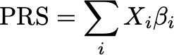
The Bayesian formulation of PRS
First, let’s frame our interpretation of the Bayesian formulation of PRS proposed by Vilhjálmsson et al. in the LDpred paper. The goal is to obtain an estimate of the true effect for each genetic variant $i$, defined as $\tilde{\beta}_i = E[\beta_i | \hat{\beta}, D]$, where $\hat{\beta}$ represents the vector of GWAS summary statistics for all observed genetic variants and D represents the LD matrix derived from population data. To compute this expectation, we define a prior distribution over $\beta$, $p(\beta|\theta)$, where $\theta$ represents our hyperparameters. Then we can obtain the resulting posterior distribution, $p(\beta | \hat{\beta}, D) = p(\hat{\beta} | \beta, D)p(\beta | \theta)$ (times a constant). Then, all we need to do is approximately compute the expectation, which can be obtained by integrating over $\beta$ or via MCMC.
Vilhjálmsson et al. solve for two cases in the LDpred paper. In the first, they let the prior on $\beta$ be a normal distribution. With this, the expectation can be computed analytically, which is quite convenient. However, the normal prior assumes that all variants have an effect on the trait (the “infinitesimal model”), which is not biologically realistic. As a result, the authors propose a sparse prior that lets variant effects be set to zero with probability p and drawn from a normal distribution with probability (1-p). This prior should be more flexible in its ability to represent many different genetic architectures. However, it does not yield a closed form solution, so LDpred employs an MCMC routine to obtain the estimates of variant effects.
Black box variational inference for PRS (bbviPRS)
Considering the Bayesian formulation from LDpred, let’s now cast this as an optimization problem using bbVI. Let $Q(\beta | \psi)$ represent our surrogate posterior distribution parameterized by $\psi$. For example, $Q$ could be a Normal distribution with mean $\mu$ and variance $\sigma^2$, in which case $\psi={\mu, \sigma^2}$. The same as above, we also define a prior over $\beta$, $p(\beta | \theta)$, where $\theta$ is our set of hyperparameters. With that, we define the ELBO in equation (2), where KL denotes the Kullback-Leibler (KL) divergence function. By maximizing the ELBO with respect to $\psi$, we are simultaneously maximizing the likelihood of our observed data (GWAS summary statistics) under the surrogate posterior while minimizing the distance of the surrogate from the prior.

From ancient statistical genetics theory, we know that $\hat{\beta}$ follows a normal distribution with mean $D\beta$ and variance $D\sigma^2$. Given that result, we can easily compute the first term in the ELBO using the normal likelihood function. For the prior, we can choose any valid probability distribution, such as the sparse prior proposed by LDpred. For the surrogate posterior Q, in theory we could also choose any distribution. In practice we rely on the mean field assumption (all variants are independent) and specify a multivariate normal distribution with mean $\alpha$ and a diagonal covariance matrix $\Psi$. We know that all variants are not independent in the posterior. In fact, we expect that their covariance is a function of LD. However, computing the true posterior covariance in the optimization is not computationally feasible, so we opt to obtain a useful approximation.
Now putting this together, the procedure for maximizing the ELBO with respect to $\psi$ using stochastic gradient descent and automatic differentiation (black box VI) is summarized in Equation (3). The idea is to sample a vector $\beta^*$ from the current surrogate and then use it to compute the ELBO. By maximizing this computed ELBO with respect to $\psi$ over samples from the surrogate, you are essentially estimating a posterior distribution that is good at creating samples of the true genetic variant effects that maximize the likelihood of the GWAS summary stats, while controlling for our prior beliefs.

Putting bbviPRS into practice with TensorFlow Probability
Probabilistic programming frameworks like TensorFlow Probability (TFP) and pyro provide language constructs that let you create probability distributions with learnable parameters and support stochastic gradient descent and automatic differentiation. What this means is that you can quite easily define loss functions like the one from Equation (3) and then run a training loop that optimizes the learnable parameters, in effect learning a probability distribution using optimization. In this section, we will show how to implement bbviPRS at a high level and then delve into some details and language constructs. However, we will attempt to keep this section brief since we are linking to a companion colab that has a full implementation with a lot of additional detail.
High level optimization routine for bbviPRS
First, let’s put the ideas we introduced above into pseudocode.
# Assume we have the following data:
#    - A vector of summary statistics - beta - length N.
#    - An NxN LD Matrix - ld_matrix.

# Sampling from the prior results in a SNP effect size vector of size M.
fixed_prior_distribution = get_my_prior(prior_hyperparams)

# Same for the posterior.
learnable_posterior_distribution = get_my_posterior()

for each optimization step:
        # Sample effect sizes from the posterior.
	beta_sample = learnable_posterior_distribution.sample()

	# Transform into GWAS summary stat space.
	beta_transform = matrix_multiply(ld_matrix, beta_sample)

	# Compute the loss as a function of the MSE between
        # the observed summary stats (beta) and the estimates
        # plus a KL-divergence term to provide regularization.
	loss = mean_squared_error(beta, beta_transform)
	# Weight the KL term inversely proportional to the data size.
	loss = loss + KL_WEIGHT * kl_divergence(
                   learnable_posterior_distribution,
                   fixed_prior_distribution)

	# Use SGD to update the learnable parameters in your posterior.
        update_estimates(loss, learnable_posterior_distribution)
Implementing bbviPRS in TensorFlow Probability
Next, let’s see how we can translate this pseudocode into working TFP code. The first idea is that TFP lets you create probability distribution objects. These objects can be used to sample from the distribution, compute probabilities and do much of the manipulations that you might do in math but using code (e.g. compute KL-divergence for two distributions). Here is the simplest example of creating a “normal prior” and plotting some samples from it.
import tensorflow as tf
import tensorflow_probability as tfp
import matplotlib.pyplot as plt

tfd = tfp.distributions

normal_prior = tfd.Normal(loc=0.0, scale=1.0)
_=plt.figure(figsize=(10,8))
normal_prior_sample = normal_prior.sample(1000).numpy()
_=plt.hist(normal_prior_sample, 100)
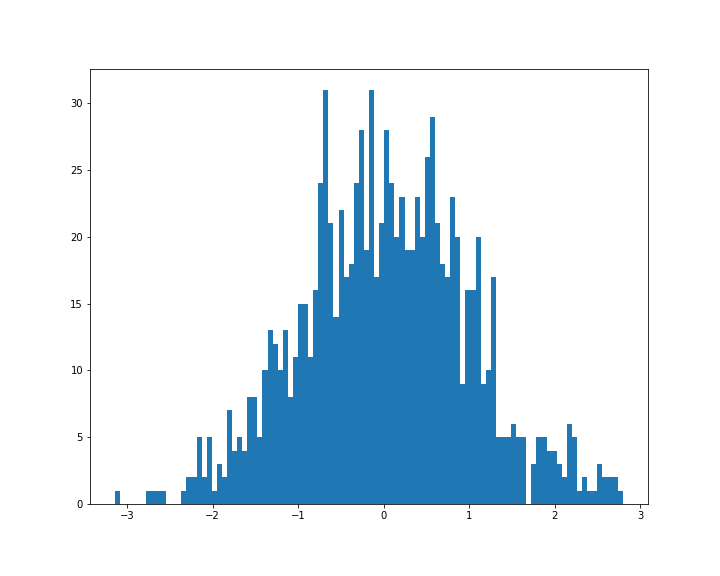
From this, hopefully you can see how we are able to define the get_my_prior function from the pseudocode above. In bbviPRS we don’t use the normal prior, but instead use a mixture of normals, where one distribution has small variance and mean zero. This distribution is similar to the sparsity inducing distribution used by LDpred. You can check the colab for implementation details.
From the prior example, there is one thing missing. We also need to introduce learnable parameters, so that we can learn our surrogate. This code snippet shows how we do that in principle.
posterior = tfd.Normal(
 loc=tf.Variable(0.0, name='posterior_mean'),
 scale=tfp.util.TransformedVariable(1.0,
                                    bijector=tfp.bijectors.Exp(),
                                    name='posterior_scale'))
Here, we create a normal distribution just as before, but we let the mean and scale parameters be represented by TFP variable objects. When we use this distribution inside of a training loop, we can specify that these parameters should be updated as part of the optimization routine.
From these basic examples, hopefully you get a sense of how we can construct and use probability distributions in our optimization code. The remaining elements from the pseudocode above are in principle pretty straightforward. Please take a look at the colab to understand more details.
A few results
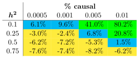
We first compared bbviPRS to LDpred2 on simulated data to get a sense of how well bbviPRS performs in terms of predictive power when compared with a known standard. We compare the Pearson correlations between the estimated PRS and the simulated phenotype in a held out test set. Phenotypes were simulated across a range of heritabilities and causal fractions. In most cases, LDPred2 appears to perform better than bbviPRS in terms of predictive power. This result is shown in Figure 1, where we report the percentage increase in Pearson correlation when using bbviPRS over LDPred2. However, for a subset of simulations, bbviPRS significantly outperforms LDPred2. Overall, bbviPRS tends to perform better than LDPred2 when heritability is small or when the fraction of causal variants is high, and does especially well when both of those two conditions hold.
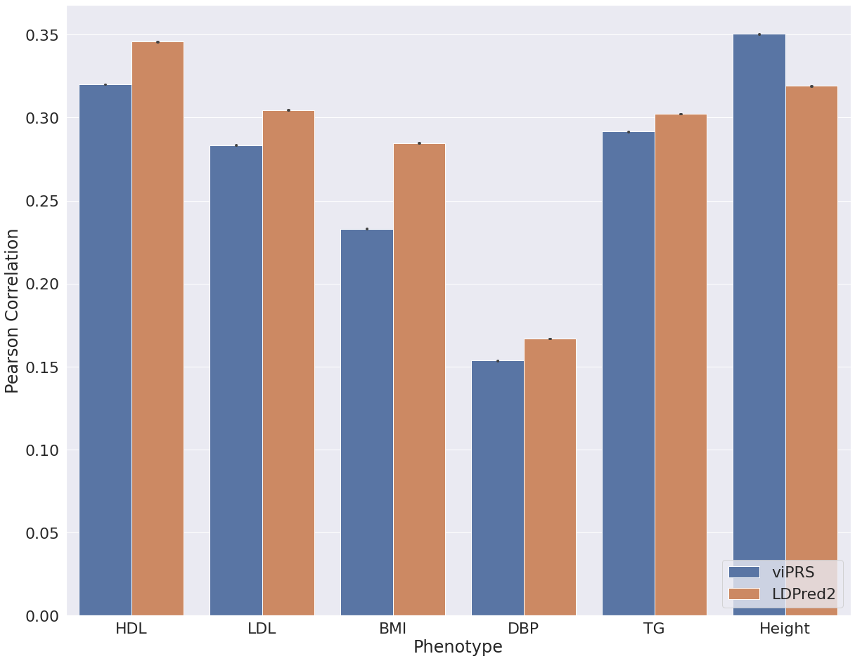
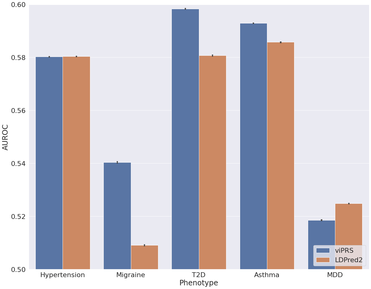
After interrogating performance on simulated data we applied bbviPRS and LDpred2 to a set of phenotypes from UK Biobank. We restricted our analysis to individuals of European ancestry, used 15 genetic PCs to control for population structure and used PLINK for association analysis with default covariates age and sex. We selected six continuous traits and five binary traits, applied each method to construct a PRS from summary statistics and then compared the predictive performance. Figure 2 shows the results for all continuous traits, where we assess the Pearson correlation between the predicted PRS and the true trait values in a hold out test set. We see that bbviPRS performs comparably with LDpred2 for some traits, but is significantly outperformed for others. In Figure 3, we assess AUROC for a set of binary traits and see that bbviPRS appears to have an advantage over LDpred2, outperforming in the majority of cases.
Final Thoughts
Here, we introduced the new idea of applying black box variational inference to the problem of estimating genetic variant effect sizes from GWAS summary statistics to construct a polygenic risk score. We showed how to derive the basic black box VI algorithm for this problem and then showed how this could be implemented in Tensorflow Probability. Finally, we show some preliminary results in both simulated and real genetic and phenotypic data.
The main advantage of the bbviPRS method is that it is extremely flexible and extensible. This means that it can give the practitioner a large degree of control and flexibility when trying new methodological ideas or incorporating new types of data. For example, you could imagine how the flexibility of bbviPRS could be an asset for models that incorporate data across different diseases or different genetic ancestries. However, the drawback to this flexibility and extensibility comes (perhaps) at the expense of predictive power. That is, as both our simulated data and many of our real data examples show, bbviPRS tends to underperform relative to LDpred2 for the baseline PRS problem.
All of that being said, we think that the black box methods laid out here could be quite useful to the statistical genetics community, so we hope this blog post and the accompanying colab can be an asset for those working in the PRS space. Good luck! Let us know how it goes.
Acknowledgements
This was joint work with Thomas Colthurst with lots of input and help from Farhad Hormozdiari, Ted Yun and Cory McLean. Special thanks to Justin Cosentino for important contributions to the infrastructure and codebase that enabled this work and results. And thanks to the entire Genomics team at Google HealthAI.
This research has been conducted using the UK Biobank Resource under Application Number 65275.