Neural Machine Translation Background

This tutorial is not meant to be a general introduction to Neural Machine Translation and does not go into detail of how these models works internally. For more details on the theory of Sequence-to-Sequence and Machine Translation models, we recommend the following resources:

• Neural Machine Translation and Sequence-to-sequence Models: A Tutorial (Neubig et al.)
• Neural Machine Translation by Jointly Learning to Align and Translate (Bahdanau et al.)
• Tensorflow Sequence-To-Sequence Tutorial

Data Format

A standard format used in both statistical and neural translation is the parallel text format. It consists of a pair of plain text with files corresponding to source sentences and target translations, aligned line-by-line. For example,

sources.en (English):

Madam President, I should like to draw your attention to a case in which this Parliament has consistently shown an interest.
It is the case of Alexander Nikitin.

targets.de (German):

Frau Präsidentin! Ich möchte Sie auf einen Fall aufmerksam machen, mit dem sich dieses Parlament immer wieder befaßt hat.
Das ist der Fall von Alexander Nikitin.

Each line corresponds to a sequence of tokens, separated by spaces. In the simplest case, the tokens are the words in the sentence. Typically, we use a tokenizer to split sentences into tokens while taking into account word stems and punctuation. For example, common choices for tokenizers are the Moses tokenizer.perl script or libraries such a spaCy, nltk or Stanford Tokenizer.

However, learning a model based on words has a couple of drawbacks. Because NMT models output a probability distribution over words, they can became very slow with large number of possible words. If you include misspellings and derived words in your vocabulary, the number of possible words is essentially infinite and we need to impose an artificial limit of how of the most common words we want our model to handle. This is also called the vocabulary size and typically set to something in the range of 10,000 to 100,000. Another drawback of training on word tokens is that the model does not learn about common "stems" of words. For example, it would consider "loved" and "loving" as completely separate classes despite their common root.

One way to handle an open vocabulary issue is learn subword units for a given text. For example, the word "loved" may be split up into "lov" and "ed", while "loving" would be split up into "lov" and "ing". This allows to model to generalize to new words, while also resulting in a smaller vocabulary size. There are several techniques for learning such subword units, including Byte Pair Encoding (BPE), which is what we used in this tutorial. To generate a BPE for a given text, you can follow the instructions in the official subword-nmt repository:

# Clone from Github
git clone https://github.com/rsennrich/subword-nmt
cd subword-nmt

# Learn a vocabulary using 10,000 merge operations
./learn_bpe.py -s 10000 < train.tok > codes.bpe

# Apply the vocabulary to the training file
./apply_bpe.py -c codes.bpe < train.tok > train.tok.bpe

After tokenizing and applying BPE to a dataset, the original sentences may look like the following. Note that the name "Nikitin" is a rare word that has been split up into subword units delimited by @@.

Madam President , I should like to draw your attention to a case in which this Parliament has consistently shown an interest .
It is the case of Alexander Ni@@ ki@@ tin .

Frau Präsidentin ! Ich möchte Sie auf einen Fall aufmerksam machen , mit dem sich dieses Parlament immer wieder befaßt hat .
Das ist der Fall von Alexander Ni@@ ki@@ tin

Download Data

To make it easy to get started we have prepared an already pre-processed dataset based on the English-German WMT'16 Translation Task. To learn more about how the data was generated, you can take a look at the wmt16_en_de.sh data generation script. The script downloads the data, tokenizes it using the Moses Tokenizer, cleans the training data, and learns a vocabulary of ~32,000 subword units.

• Download pre-processed WMT'16 EN-DE Data (502MB)

After extraction, you should see the folowing files:

Filename	Description
train.tok.clean.bpe.32000.en	The English training data, one sentence per line, processed using BPE.
train.tok.clean.bpe.32000.de	The German training data, one sentence per line, processed using BPE.
vocab.bpe.32000	The full vocabulary used in the training data, one token per line.
newstestXXXX.*	Development and test data sets, in the same format as the training data. We provide both pre-processed and original data files used for evaluation.

Let's set a few data-specific environment variables so that we can easily use them later on:

# Set this to where you extracted the downloaded file
export DATA_PATH=

export VOCAB_SOURCE=${DATA_PATH}/vocab.bpe.32000
export VOCAB_TARGET=${DATA_PATH}/vocab.bpe.32000
export TRAIN_SOURCES=${DATA_PATH}/train.tok.clean.bpe.32000.en
export TRAIN_TARGETS=${DATA_PATH}/train.tok.clean.bpe.32000.de
export DEV_SOURCES=${DATA_PATH}/newstest2013.tok.bpe.32000.en
export DEV_TARGETS=${DATA_PATH}/newstest2013.tok.bpe.32000.de

export DEV_TARGETS_REF=${DATA_PATH}/newstest2013.tok.de
export TRAIN_STEPS=1000000

Alternative: Generate Toy Data

Training on real-world translation data can take a very long time. If you do not have access to a machine with a GPU but would like to play around with a smaller dataset, we provide a way to generate toy data. The following command will generate a dataset where the target sequences are reversed source sequences. That is, the model needs to learn the reverse the inputs. While this task is not very useful in practice, we can train such a model quickly and use it as as sanity-check to make sure that the end-to-end pipeline is working as intended.

DATA_TYPE=reverse ./bin/data/toy.sh

Instead of the translation data, use the files generated by the script:

export VOCAB_SOURCE=${HOME}/nmt_data/toy_reverse/train/vocab.sources.txt
export VOCAB_TARGET=${HOME}/nmt_data/toy_reverse/train/vocab.targets.txt
export TRAIN_SOURCES=${HOME}/nmt_data/toy_reverse/train/sources.txt
export TRAIN_TARGETS=${HOME}/nmt_data/toy_reverse/train/targets.txt
export DEV_SOURCES=${HOME}/nmt_data/toy_reverse/dev/sources.txt
export DEV_TARGETS=${HOME}/nmt_data/toy_reverse/dev/targets.txt

export DEV_TARGETS_REF=${HOME}/nmt_data/toy_reverse/dev/targets.txt
export TRAIN_STEPS=1000

Defining the model

With the data in place, it is now time to define what type of model we would like to train. The standard choice is a Sequence-To-Sequence model with attention. This type of model has a large number of available hyperparameters, or knobs you can tune, all of which will affect training time and final performance. That's why we provide example configurations for small, medium, and large models that you can use or extend. For example, the configuration for the medium-sized model look as follows:

model: AttentionSeq2Seq
model_params:
  attention.class: seq2seq.decoders.attention.AttentionLayerBahdanau
  attention.params:
    num_units: 256
  bridge.class: seq2seq.models.bridges.ZeroBridge
  embedding.dim: 256
  encoder.class: seq2seq.encoders.BidirectionalRNNEncoder
  encoder.params:
    rnn_cell:
      cell_class: GRUCell
      cell_params:
        num_units: 256
      dropout_input_keep_prob: 0.8
      dropout_output_keep_prob: 1.0
      num_layers: 1
  decoder.class: seq2seq.decoders.AttentionDecoder
  decoder.params:
    rnn_cell:
      cell_class: GRUCell
      cell_params:
        num_units: 256
      dropout_input_keep_prob: 0.8
      dropout_output_keep_prob: 1.0
      num_layers: 2
  optimizer.name: Adam
  optimizer.learning_rate: 0.0001
  source.max_seq_len: 50
  source.reverse: false
  target.max_seq_len: 50

You can write your own configuration files in YAML/JSON format, overwrite configuration values with another file, or pass them directly to the training script. We found that saving configuration files is useful for reproducibility and experiment tracking.

Training

Now that we have both a model configuration and training data we can start the actual training process. On a single modern GPU (e.g. a TitanX), training to convergence can easily take a few days for the WMT'16 English-German data, even with the small model configuration. We found that the large model configuration typically trains in 2-3 days on 8 GPUs using distributed training in Tensorflow. The toy data should train in ~10 minutes on a CPU, and 1000 steps are sufficient.

export MODEL_DIR=${TMPDIR:-/tmp}/nmt_tutorial
mkdir -p $MODEL_DIR

python -m bin.train \
  --config_paths="
      ./example_configs/nmt_small.yml,
      ./example_configs/train_seq2seq.yml,
      ./example_configs/text_metrics_bpe.yml" \
  --model_params "
      vocab_source: $VOCAB_SOURCE
      vocab_target: $VOCAB_TARGET" \
  --input_pipeline_train "
    class: ParallelTextInputPipeline
    params:
      source_files:
        - $TRAIN_SOURCES
      target_files:
        - $TRAIN_TARGETS" \
  --input_pipeline_dev "
    class: ParallelTextInputPipeline
    params:
       source_files:
        - $DEV_SOURCES
       target_files:
        - $DEV_TARGETS" \
  --batch_size 32 \
  --train_steps $TRAIN_STEPS \
  --output_dir $MODEL_DIR

Let's look at the training command in more detail and explore what each of the options mean.

• The config_paths argument allows you to pass one or more configuration files used for training. Configuration files are merged in the order they are specified, which allows you to overwrite specific values in your own files. Here, we pass two configuration files. The file nmt_small.yml contains the model type and hyperparameters (as explained in the previous section) and train_seq2seq.yml contains common options about the training process, such as which metrics to track, and how often to sample responses.
• The model_params argument allows us to overwrite model parameters. It is YAML/JSON string. Most of the parameters are defined in the nmt_small.yml file, but since the vocabulary depends on the data we are using, we need to overwrite it from the command line.
• The input_pipeline_train and input_pipeline_dev arguments define how to read training and development data. In our case, we use a parallel text format. Note that you would typically define these arguments in the configuration file. We don't do this in this tutorial because the path of the extracted data depends on your local setup.
• The output_dir is the desination directory for model checkpoints and summaries.

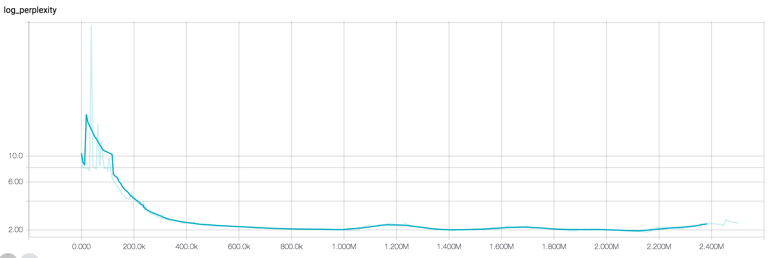
Throughout the traning process you will see the loss decreasing and samples generated by the model. To monitor the training process, you can start Tensorboard pointing to the output directory:

tensorboard --logdir $MODEL_DIR

Making predictions

Once your model is trained, you can start predictions, i.e. translating new data from German to English. For example:

export PRED_DIR=${MODEL_DIR}/pred
mkdir -p ${PRED_DIR}

python -m bin.infer \
  --tasks "
    - class: DecodeText" \
  --model_dir $MODEL_DIR \
  --input_pipeline "
    class: ParallelTextInputPipeline
    params:
      source_files:
        - $DEV_SOURCES" \
  >  ${PRED_DIR}/predictions.txt

Let's take a closer look at this command again:

• The tasks argument specifies which inference tasks to run. It is a YAML/JSON string, containing a list of class names and optional parameters. In our command, we only execute the DecodeText task, which takes the model predictions and prints them to stdout. Other possible tasks include DumpAttention or DumpBeams, which can be used to write debugging information about what your model is doing. For more details, refer to the Inference section.
• The model_dir argument points to the path containing the model checkpoints. It is the same as the output_dir passed during training.
• input_pipeline defines how we read data and is of the same format as the input pipeline definition used during training.

Decoding with Beam Search

Beam Search is a commonly used decoding technique that improves translation performance. Instead of decoding the most probable word in a greedy fashion, beam search keeps several hypotheses, or "beams", in memory and chooses the best one based on a scoring function. To enable beam search decoding, you can overwrite the appropriate model parameter when running inference. Note that decoding with beam search will take significantly longer.

python -m bin.infer \
  --tasks "
    - class: DecodeText
    - class: DumpBeams
      params:
        file: ${PRED_DIR}/beams.npz" \
  --model_dir $MODEL_DIR \
  --model_params "
    inference.beam_search.beam_width: 5" \
  --input_pipeline "
    class: ParallelTextInputPipeline
    params:
      source_files:
        - $DEV_SOURCES" \
  > ${PRED_DIR}/predictions.txt

The above command also demonstrates how to pass several tasks to the inference script. In our case, we also dump beam search debugging information to a file on disk so that we can inspect it later.

Evaluating specific checkpoint

The training script will save multiple model checkpoints throughout training. The exact checkpoint behavior can be controlled via training script flags. By default, the inference script evaluates the latest checkpoint in the model directory. To evaluate a specific checkpiint you can pass the checkpoint_path flag.

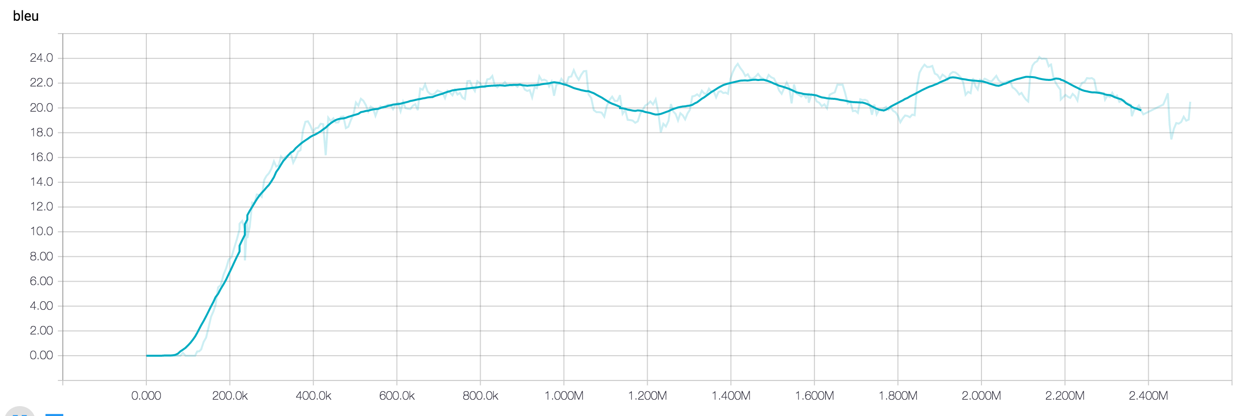
Calcuating BLEU scores

BLEU is a commonly used metric to evaluate translation performance. Now that you have generated prediction in plain text format, you can evaluate your translations against the reference translations using BLEU scores:

./bin/tools/multi-bleu.perl ${DEV_TARGETS_REF} < ${PRED_DIR}/predictions.txt

The multi-bleu.perl script is taken from Moses and is one of the most common ways to calculcate BLEU. Note that we calculate BLEU scores on tokenized text. An alternative is to calculate BLEU on untokenized text. To do this, would first need to detokenize your model outputs.