Delay Estimation Methodology

Context

This doc describes the delay estimation methodology used in XLS and related background.

Estimating delays through networks of CMOS gates is a rich topic, and Static Timing Analysis (STA) is used in chip backend flows to ensure that, even for parts operating at the tail end of the distribution, chips continue to function as specified logically in the netlist.

In stark contrast to something with very concrete constraints, like a "post-global routing, high-accuracy parasitics static timing analysis", the HLS tool needs to estimate at a high level, reasonably near to the user's behavioral specification, what delay HLS operations will have when they are "stacked on top" of each other in a data dependent fashion in the design.

This information lets the HLS tool schedule operations into cycles without violating timing constraints; e.g. if the user specifies 1GHz (= 1000ps) as their target clock frequency, the HLS tool may choose to pack as much data dependent work into the 1000ps budget (minus clock uncertainty) as it can on any given cycle.

Although what we're estimating is a close relative of Static Timing Analysis, the fact it's being analyzed at a very high level presents a different set of tradeoffs, where coarse granularity estimation and conservative bounds are more relevant. Fine-grained / precise analyses are used later in the chip design process, in the backend flows, but the HLS tool acts more like an RTL designer, creating an RTL output that early timing analysis deems acceptable.

Notably, we don't want to be too conservative, as being conservative on timing can lead to designs that take more area and consume more power, as the flops introduced by additional pipeline stages are significant. We want to be as accurate as possible while providing a good experience of being able to close timing quickly (say, in a single pass, or with a small number of iterations in case of a pathological design).

Background

What XLS is compiling

XLS currently supports feed-forward pipelines -- once the user program is unrolled into a big "sea of nodes" we must schedule each of those operations (represented by nodes) to occur in a cycle.

It seems clear that an operation like add(bits[32], bits[32]) -> bits[32] takes some amount of time to produce a result -- we need to be able to determine what that amount of time is for packing that operation into a given cycle. ¹ Note that XLS operations are parametric in their bitwidth, so add(bits[17], bits[17]) -> bits[17] is just as possible as a value like 32. This ain't C code.

1: Note that we currently pack operations into cycles atomically -- that is, we don't break an add that would straddle a cycle boundary into add.first_half and add.second_half automatically to pull things as early as possible in the pipeline, but this is future work of interest. Ideally operations would be described structurally in a way that could automatically be cut up according to available delay budget. This would also permit operations in the IR that take more than a single cycle to produce a value (currently they would have to be "legalized" into operations that fit within a cycle, but that is not yet done, the user will simply receive a scheduling error).

Some operations, such as bit_slice or concat are just wiring "feng shui"; however, they still have some relevance for delay calculations! Say we concatenate a value with zeros for zero extension. Even if we could schedule that in "cycle 0", if the consumer can only be placed in "cycle 1", we would want to "sink" the concat down into "cycle 1" as well to avoid unnecessary registers being materialized sending the zero values from "cycle 0".

The delay problem

Separately from XLS considerations, there are fundamental considerations in calculating the delay through clouds of functional logic in (generated) RTL.

Between each launching and capturing flop is a functional network of logic gates, implemented with standard cells in our ASIC process flows. Chip designs target a particular clock frequency as their operating point, and the functional network has to produce its output value with a delay that meets the timing constraint of the clock frequency. The RTL designer typically has to iterate their design until:

timing path delay <= target clock period - clock uncertainty

For all timing paths in their design, where clock uncertainty includes setup/hold time constraints, and slop that's built in as margin for later sources of timing variability (like instantiating a clock tree, which can skew the clock signal observed by different flops).

In a reasonable model, gate delay is affected by a small handful of properties, as reflected in the "(Method of) Logical Effort" book:

• The transistor network used to implement a logic function (AKA logical effort): on an input pin change, the gate of each transistor must be driven to a point it recognizes whether a 0 or 1 voltage is being presented. More gates to drive, or larger gates, means more work for the driver.
• The load being driven by the logic function (AKA electrical effort): fanning out to more gates generally means more work to drive them all to their threshold voltages. Being loaded down by bigger gates means more work to drive it to its threshold voltage.
• Parasitic delays: RC elements in the system that leech useful work, typically in a smaller way compared to the efforts listed above.

The logical effort book describes a way to analyze the delays through a network of gates to find the minimal delay, and size transistors in a way that can achieve that minimal delay (namely by geometrically smoothing the ability for gate to drive capacitance).

Confounding factors include:

• Medium/large wires: sizing transistors to smooth capacitance becomes difficult as fixed-capacitance elements (wires) are introduced. It seems that small wires have low enough capacitance they can generally be treated as parasitic.
• Divergence/reconvergence in the functional logic network (as a DAG). Different numbers of logic levels and different drive currents may be presented from different branches of a fork/join the logic graph, which forces delay analysis into a system of equations to attempt to minimize the overall delay, as observed by the critical path, with transistor sizing and gate choices. (Some simplifications are possible, like buffering non-critical paths until they have the same number of logic levels so they also have plenty of current to supply at join points.)

Somewhat orthogonal to the analytical modeling problem, there are also several industry standards for supplying process information to Static Timing Analysis engines for determining delay through a netlist. This information is often given in interpolated tables for each standard cell, for example in the NLDM model describing how delay changes as a function of input transition time and load (load capacitance).

These models and supplied pieces of data are important to keep in mind for contrast, as we now ignore it all and do something very simple.

Simple Delay Estimation

Currently, XLS delay estimation follows a conceptually simple procedure:

• For every operation in XLS (e.g. binary addition):

  • For some relevant-seeming set of bitwidths; e.g. {2, 4, 8, 16, ..., 2048}
  • Find the maximum frequency at which that operation closes timing at that bitwidth, in 100MHz units as determined by the synthesis tool. ² Call the clock period for this frequency t_best. (Note that we currently just use a single process corner / voltage for this sweep.)
  • Subtract the clock uncertainty from t_best.
  • Record that value in a table (with the keys of the table being operation / bitwidth).

2: The timing report can provide the delay through a path at any clock frequency, but a wrinkle is that synthesis tools potentially only start using their more aggressive techniques as you bump up against the failure-to-close-timing point -- there it'll be more likely to change the structure of the design to make it more delay friendly. The sweep helps to try to cajole it in that way.

Inspecting the data acquired in this way we observe all of the plots consist of one or more the following delay components:

• Constant as a function of bitwidth for a given op (e.g. binary-or just requires a single gate for each bit regardless of the width of the inputs).
• Logarithmic as a function of bitwidth (e.g. adders may end up using tree-like structures to minimize delay, single-selector muxes end up using a tree to fan out the selector to the muxes, etc.).
• Linear as a function of bitwidth (e.g., ripple-carry adders and some components of multipliers).

So given this observation we fit a curve of the form:

a * bitwidth + b * log_2(bitwidth) + c

to the sweep data for each operation, giving us (a, b, c) values to use in our XLS delay estimator.

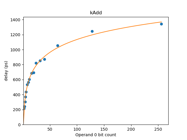
The utility delay_model_visualizer under the tools directory renders a graph of the delay model estimate against the measured data points. This graph for add shows a good correspondence to the measured delay.

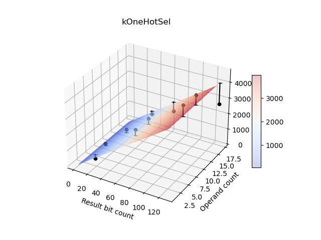
Sweeping multiple dimensions

Operations with attributes in addition to bitwidth that affect delay are swept across multiple dimensions. An example is Op::kOneHotSelect which has dimensions of bitwidth and number of cases. For the Op::kOneHotSelect example the formula is:

a * bitwidth + b * log_2(bitwidth) + c * (# of cases) + d * log_2(# of cases) + c

Below is plot of delay for Op::kOneHotSelect showing the two dimensions of bitwidth and operand count affecting delay:

Sources of pessimism/optimism

This simple method has both sources of optimism and pessimism, though we hope to employ a method that will be generally conservative, so that users can easily close timing and get a close-to-best-achievable result (say, within tens of percent) with a single HLS iteration.

Sources of pessimism (estimate is conservative):

• The operation sweeps mentioned are not bisecting to the picosecond, so there is inherent slop in the measurement on account of sweep granularity.
• We expect, in cycles where multiple dependent operations are present, there would be "K-map style" logic reductions with adjacent operations. For example, because we don't do cell library mapping in XLS delay estimation, something a user wrote that mapped to an AOI21 cell would be the sum of (and+or+invert) delays.
• [Unsure] May there be additional logic branch splitting options and earlier-produced results available to the synthesis tool when there are more operations in the graph (vs a lone critical path measured for a single operation)?

Sources of optimism (estimate is overeager):

• For purposes of the sweep the outputs of an operation are only loaded by a single capture flop flop -- when operations have fanout the delay will increase.

  Note that we do account for fanout within individual operations as part of this sweep; e.g. a 128-bit selector fanout (e.g. 128 ways to 128 muxes) for a select is accounted for the in delay timing of the select operation. It is the output logic layer that is only loaded by a single flop in our characterization. Notably because most of these operations turn into trees of logic, there are \(\(log_2(bitcount)\)\) layers of logic in which we can potentially smoothly increase drive strength out to the output logic layer, and paths can presumably be replicated by synthesis tools to reduce pointwise fanout when multiple high-level operations are data-dependent within a cycle. (Is it possible for a user to break up their 32-bit select into bitwise pieces in their XLS code to mess with our modeling? Sure, but probably not too expected, so we're currently sort of relying on the notion people are using high level operations instead of compodecomposing them into bitwise pieces in our graph.)

  A potential way to reconcile this output fanout in the future is to do a delay sweep with a high-capacitive fanout (e.g. four flops of load) and then ensure the IR has a maximum fanout of four for our delay estimation.

• Wiring delay / load / congestion / length are not estimated. This will need additional analysis / refinement as we run XLS through synthesis tools with advanced timing analysis, as it is certainly not viable for arbitrary designs (tight pipelines may be ok for now, though).

Iterative refinement

The caveats mentioned above seem somewhat daunting, but this first cut approach appears to work comfortably at target frequenties, in practice, for the real-world blocks being designed as XLS "first samples".

Notably, human RTL designers fail to close timing on a first cut as well -- HLS estimations like the above assist in getting a numeric understanding (in lieu of an intuitive guess) of something that may close timing on a first cut. As this early model fails, we will continue to refine it; however, there is also a secondary procedure that can assist as the model improves.

Let's call the delay estimation described above applied to a program a prediction of its delays. Let's call the first prediction we make p0: p0 will either meet timing or fail to meet timing.

When we meet timing with p0, there may be additional wins left on the table. If we're willing to put synthesis tool runs "in the loop" (say running a "tuner" overnight), we can refine XLS's estimates according to the realities of the current program, and, for example, try to squeeze as much as possible into as few cycles as possible if near-optimality of latency/area/power were a large consideration. This loop would generate p1, p2, ... as it refined its model according to empirical data observed from the synthesis tool's more refined analysis.

When we fail to close timing with p0, we can feed back the negative slack delays for comparison with our estimates and relax estimates accordingly. Additionally, an "aggression" knob could be implemented that backs off delay estimations geometrically (say via a "fudge factor" coefficient) in order to ensure HLS developer time is not wasted unnecessarily to ensure. Once a combination of these mechanisms has obtained a design that closes timing, the "meeting timing, now refine" procedure can be employed as described above.

On Hints

To whatever extent possible, XLS should be the tool that reasons about how to target the backend (vs having a tool that sits on top of it and messes with XLS' input in an attempt to achieve a result). User-facing hint systems are typically very fragile, owing to the fact they don't have easily obeyed semantics. XLS, by contrast, knows about its own internals, so can do things with awareness of what's happened upstream and what remains to happen downstream.

By contrast, we should continue to add ways for users to provide more semantic information / intent as part of their program (e.g. via more high-level patterns that make high level structure more clear), and make XLS smarter about how to lower those constructs into hardware (and why it should be lowering them that way) in the face of some prioritized objectives (power/area/latency).

That being said, because we're probably trying to produce hardware at a given point in time against a given technology, it likely makes sense to permit human users to specify things directly (at a point in time), even if those specifications might be ignored / handled very differently in the future or against different technology nodes. This would be the moral equivalent of what existing EDA tools do as a "one-off TCL file" used in a particular design, vs something carried from design to design. Recall, though, that the intent of XLS is to make things easier to carry from design to design and require fewer one-off modifications!

Tools

XLS provides tools for analyzing its delay estimation model. (Note that the given IR should be in a form suitable for code generation; e.g. it has run through the opt_main binary).

$ bazel run -c opt //xls/dev_tools:benchmark_main -- $PWD/bazel-bin/xls/examples/crc32.opt.ir --clock_period_ps=500 --delay_model=sky130
<snip>
Critical path delay: 8351ps
Critical path entry count: 43
Critical path:
   8351ps (+ 21ps): not.37: bits[32] = not(xor.213: bits[32], id=37, pos=[(0,30,51)])
   8330ps (+128ps): xor.213: bits[32] = xor(concat.203: bits[32], and.222: bits[32], id=213, pos=[(0,25,19)])
   8202ps (+ 81ps): and.222: bits[32] = and(mask__7: bits[32], literal.395: bits[32], id=222, pos=[(0,25,33)])
   8121ps (+621ps)!: mask__7: bits[32] = neg(concat.199: bits[32], id=202, pos=[(0,24,15)])
   7330ps (+  0ps): concat.199: bits[32] = concat(literal.387: bits[31], bit_slice.198: bits[1], id=199, pos=[(0,24,21)])
   7330ps (+  0ps): bit_slice.198: bits[1] = bit_slice(xor.196: bits[32], start=0, width=1, id=198, pos=[(0,24,21)])
   7330ps (+128ps): xor.196: bits[32] = xor(concat.194: bits[32], and.221: bits[32], id=196, pos=[(0,25,19)])
   7202ps (+ 81ps): and.221: bits[32] = and(mask__6: bits[32], literal.394: bits[32], id=221, pos=[(0,25,33)])
<snip>

In addition to the critical path, the cycle-by-cycle breakdown of which operations have been scheduled is provided in stdout.